Lecture 4, ACM 11
Contents
- Making a plot with error bars
- Basic regression
- Better regression by doing it ourselves
- 3D plotting
- vector field plots
- displaying images
- Importing data the very easy way
- Sparse matrices
- Eigenvalues
- Singular Value Decomposition (SVD)
- Numerical Integration, aka quadrature
- dialog boxes, etc.
- "while" statement; "break"
- Dealing with errors
Making a plot with error bars
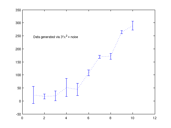
This is easy: use "errorbar" (see "help specgraph")
clear;clf;clc
x = 1:10;
randn('state',5);
y = 3*x.^2 + 20*randn(1,10);
err = 30*randn(1,10);
errorbar(x,y,err,':');  % these are just as an example; they have no real meaning
text(1,250,'Data generated via 3*x^2 + noise');
Basic regression
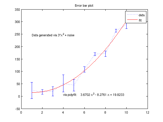
Using the data from the error-bar plot, let's fit it to a polynomial
p = polyfit(x,y,2);     % we want a degree-2 polynomial

estimate = polyval(p, 1:.1:10 );
hold on
plot(1:.1:10,estimate,'r')
legend('data','fit')
text(4,10, ['via polyfit: ' poly2str(p,'x')])
title('Error bar plot')

% You can also do this graphically; in the figure window, go to "Tools" and
% pick "Basic Fitting".
Better regression by doing it ourselves
First, we recreate the results of polyfit "by hand" For a general quadratic fit, we do the following:
x = x(:); y = y(:);   % make sure x and y are column vectors
A = [x.^0, x, x.^2 ]
coefficients = A\y    % the backslash solver minimizes the l_2 norm of the residual
% This is the same as what polyfit gave us!
A =

     1     1     1
     1     2     4
     1     3     9
     1     4    16
     1     5    25
     1     6    36
     1     7    49
     1     8    64
     1     9    81
     1    10   100


coefficients =

   19.8233
   -8.2761
    3.6702
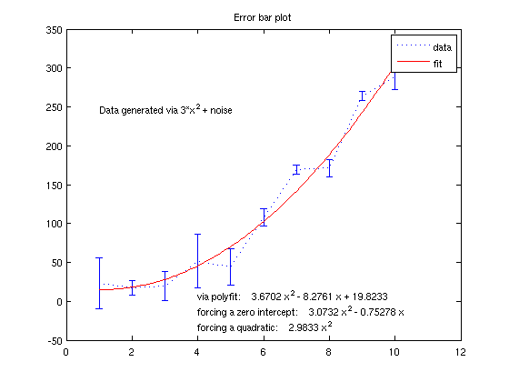
Now, suppose we know that the polynomial that best explains our data has no constant term. We can use this info to improve our estimate Now, we get rid of the 1's column:
coefficients = A(:,2:3)\y
coefficients = [flipud(coefficients);0];
text(4,-10,['forcing a zero intercept: ' poly2str(coefficients,'x')])

% And if we know it's exactly a quadratic, we would do this:
coefficients = A(:,3:3)\y
coefficients = [flipud(coefficients);0;0];
text(4,-30,['forcing a quadratic: ' poly2str(coefficients,'x')])
coefficients =

   -0.7528
    3.0732


coefficients =

    2.9833
3D plotting
Suppose we want a 3D plot of sin(x)*cos^2*(y). The simplest way to set this up is using "meshgrid".
clc;clear; N = 5;
f = @(x,y) sin(x).*(cos(y).^2);
x = linspace(0, 2*pi, N );
y = linspace(0, 2*pi, N );
[xGrid,yGrid] = meshgrid(x,y)
xGrid =

         0    1.5708    3.1416    4.7124    6.2832
         0    1.5708    3.1416    4.7124    6.2832
         0    1.5708    3.1416    4.7124    6.2832
         0    1.5708    3.1416    4.7124    6.2832
         0    1.5708    3.1416    4.7124    6.2832


yGrid =

         0         0         0         0         0
    1.5708    1.5708    1.5708    1.5708    1.5708
    3.1416    3.1416    3.1416    3.1416    3.1416
    4.7124    4.7124    4.7124    4.7124    4.7124
    6.2832    6.2832    6.2832    6.2832    6.2832
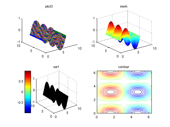
Here are four types of plots that are useful for 2D functions
N = 100;
x = linspace(0, 2*pi, N );
y = linspace(0, 2*pi, N );
[xGrid,yGrid] = meshgrid(x,y);
F = f(xGrid,yGrid);
% For 3D plotting tools, type "help graph3d"
figure(1); clf; subplot(2,2,1)
plot3(xGrid,yGrid,F,'o'); title('plot3')

subplot(2,2,2)
mesh(xGrid,yGrid,F); title('mesh') % better!

subplot(2,2,3)
surf(xGrid,yGrid,F); title('surf')
colorbar('location','westoutside')  % this adds a legend describing the
                                    % significance of each color
subplot(2,2,4)
contour(xGrid,yGrid,F,20);  title('contour');
% "contour" is listed in "help specgraph" along with many other useful
% functions

% In the figure window, click the "Rotate 3D" icon (let the mouse hover
% over the icons to see their names), and you can rotate these objects.
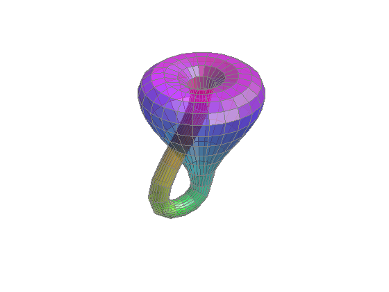
Here are some cool 3D plots that give an idea of what Matlab is capable of.
clf; xpklein
teapotdemo

transpdemo % this crashed my computer!
volvec % this behaves funny too, but gives an idea of how to display 3D stream lines. type "edit volvec" for details.
vector field plots
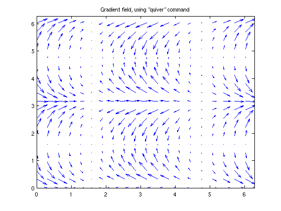
If you have the values of the vectors, then something like "quiver" will do what you want. Take our function "f" from earlier, and find the gradient field.
dfdx = @(x,y) cos(x).*(cos(y).^2);
dfdy = @(x,y) -2*cos(x).*cos(y).*sin(y);
% let's make a smaller grid so that it's not too crowded
close;clf;[xGrid,yGrid] = meshgrid(x(1:5:end),y(1:5:end));
quiver(xGrid,yGrid,dfdx(xGrid,yGrid), dfdy(xGrid,yGrid) )
title('Gradient field, using "quiver" command')
xlim([0,2*pi]); ylim([0,2*pi]);
displaying images
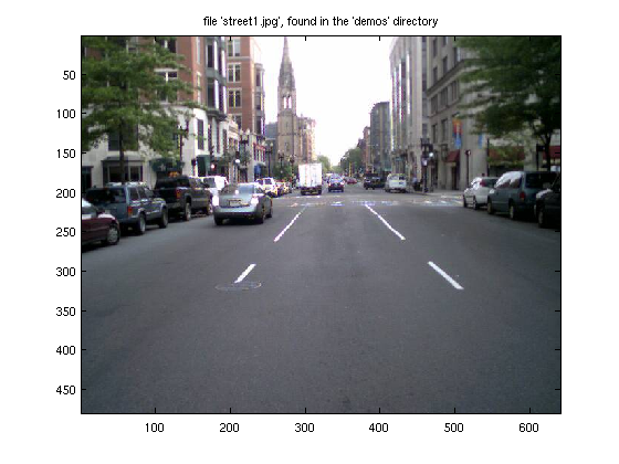
Matlab can display most common image file formats, including jpeg. To see all the availabe functions, type "help specgraph" and see the "Images display and file I/O" section. The basic command to load an image is "imread()". This will open the file and convert it to either a 2D array, or a 3D array if it has color. The 3D array will basically have 3 copies of the 2D array, with each copy representing a different color (these do not have to be colors -- they could be chrominance, luminance, etc.; often, these are referred to as "channels"). The data in the array will probably be an unsigned integer, and not a floating point number; this is done to keep the RAM requirements as small as possible. It's always possible to convert back to to a floating point number using "double()", but if you just want to display the image, this is unnecessary, because the display functions expect unsigned integer datatypes.
% This file should be on everyone's computer
% (type "which street1.jpg" to see where it's located)
clear; X = imread('street1','jpeg');
% X = imread('street1.jpg');    % this command work work also
whos X
% We see that X is a 3D array, with type "unsigned integer, 8 bits"
  Name      Size                           Bytes  Class

  X       480x640x3                       921600  uint8 array

Grand total is 921600 elements using 921600 bytes
To actually view the image, we can use "image" or "imagesc". "imagesc" is identical to "image", except that the values will be scaled to take up the full range of colors available. If you need to convert something back to an integer form, use "uint8()". To see all possible conversions, type "help datatypes" and "help isa"
imagesc(X); title(' file ''street1.jpg'', found in the ''demos'' directory');
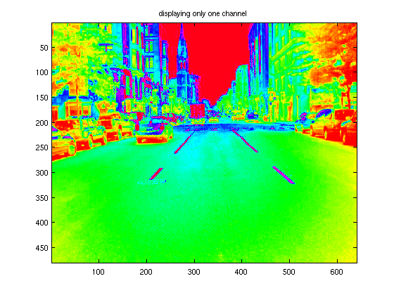
We can view only one channel of the image, if we wish
imagesc( X(:,:,1) ); title('displaying only one channel');
Importing data the very easy way
Use Matlab's graphical importer:
uiimport
Also, here's a useful function to see what variables are inside a .mat file (in this example, there's a file called "myFile.mat")
whos -file myFile
% and a nice way to see (and modify) the values if a variable is with the
% "openvar" command.
s = randn(9,1);
openvar s       % the form   openvar('s')   also works
  Name            Size                    Bytes  Class

  variable1       1x1                         8  double array
  variable2       1x3                        24  double array

Grand total is 4 elements using 32 bytes
Sparse matrices
In a few fields, the term "sparse" has become a buzzword. What does it mean? There's no quantitative definition, but the qualitative definition is easy: a vector or matrix is "sparse" when it has many zero entries. In Matlab, there are two ways to store a matrix. The first way, which we've been using so far, is to store all entries. If we know the dimensions of the matrix, and have a convention of how the entries are stored, then there is no need to store the indices. The second method, which Matlab calls the "sparse" datatype, is to only store the nonzero entries. But, with this scheme, we need to store the indices also, so there's a penalty in memory. It is very important to realize that Matlab's definition of "sparse" only refers to the way a matrix is stored. The same matrix can be sparse, or non-sparse (aka "full"). Here's an example:
clc; clear;
A = randn(5)        % Method 1 of storing a matrix, aka "full" storage
B = sparse(A)       % Method 2 of storing a matrix, aka "sparse" storage
% The "sparse" function converts a matrix to the sparse storage format.  We
% can go the other direction using the "full" command, e.g.
% A = full(B);
A =

    0.5777    0.7453   -0.6938    0.2237   -1.1142
    1.6701   -0.5550    0.7174    1.4295   -0.2797
   -0.2803   -0.0587   -0.5504    1.5706    0.9893
    0.9819    0.8630   -1.7900    1.4769   -0.7902
   -0.7271   -1.3078    1.3686   -1.1266   -1.1000


B =

   (1,1)       0.5777
   (2,1)       1.6701
   (3,1)      -0.2803
   (4,1)       0.9819
   (5,1)      -0.7271
   (1,2)       0.7453
   (2,2)      -0.5550
   (3,2)      -0.0587
   (4,2)       0.8630
   (5,2)      -1.3078
   (1,3)      -0.6938
   (2,3)       0.7174
   (3,3)      -0.5504
   (4,3)      -1.7900
   (5,3)       1.3686
   (1,4)       0.2237
   (2,4)       1.4295
   (3,4)       1.5706
   (4,4)       1.4769
   (5,4)      -1.1266
   (1,5)      -1.1142
   (2,5)      -0.2797
   (3,5)       0.9893
   (4,5)      -0.7902
   (5,5)      -1.1000
If we look at the memory of the two variables, we see that the sparse datatype takes more memory, because we also have to store the coordinates.
whos
  Name      Size                    Bytes  Class

  A         5x5                       200  double array
  B         5x5                       324  double array (sparse)

Grand total is 50 elements using 524 bytes
Now, suppose we have a matrix that really is sparse. THEN the sparse matrix format has the advantage:
clear; A = zeros(100);
A(45,60) = 1;  % method 1
B = sparse(A)  % method 2
whos
B =

  (45,60)       1

  Name      Size                    Bytes  Class

  A       100x100                   80000  double array
  B       100x100                     416  double array (sparse)

Grand total is 10001 elements using 80416 bytes
We can create a sparse matrix on its own, i.e. we don't have to convert from a full matrix first. The simplest method is the following:
clear;
B = sparse(100,100); % makes an empty 100 x 100 sparse matrix
% Note: B = sparse(100) is NOT what you want.  This would make a 1 x 1 sparse
% matrix, with the (1,1) entry being 100.

B(45,60) = 4
B =

  (45,60)       4
Just like with the default matrix storage, we can "expand" a sparse matrix after we define it, and this also penalizes us in terms of memory (since we have to re-allocate space in RAM every time we extend the matrix). We can allocate memory and define a sparse matrix all at once, again using the "sparse" command. Here's an example:
clear;
A = rand(45,50);   % uniform random numbers in [0,1]
[i,j,s] = find( A .* (A < .01)  );
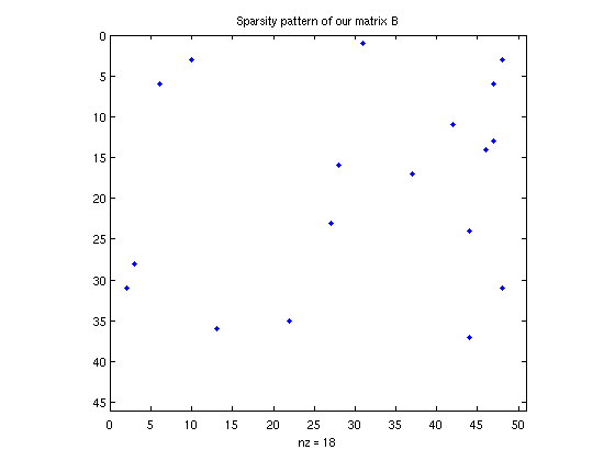
B = sparse(i,j,s,45,50)
B =

  (31,2)       0.0021
  (28,3)       0.0060
   (6,6)       0.0092
   (3,10)      0.0096
  (36,13)      0.0081
  (35,22)      0.0020
  (23,27)      0.0100
  (16,28)      0.0046
   (1,31)      0.0079
  (17,37)      0.0053
  (11,42)      0.0043
  (24,44)      0.0007
  (37,44)      0.0024
  (14,46)      0.0018
   (6,47)      0.0097
  (13,47)      0.0024
   (3,48)      0.0014
  (31,48)      0.0090
Some useful functions for sparse matrices (type "help sparfun" for a full list).
% Visualize the sparsity pattern.
spy(B); title('Sparsity pattern of our matrix B');
% How many non-zero entries:
fprintf('matrix B has %d nonzero entries\n', nnz(B) );
% Is the matrix stored in the sparse format?  (note: this does NOT imply
% that the matrix really is sparse, only that it is stored in the sparse
% format).
fprintf('matrix A is sparse?  %d\n', issparse(A) );
fprintf('matrix B is sparse?  %d\n', issparse(B) );
matrix B has 18 nonzero entries
matrix A is sparse?  0
matrix B is sparse?  1
Eigenvalues
Matlab has a good eigenvalue solver called "eig". This is different than "eigs" (which we will cover in a minute; the "s" stands for "sparse", and not to pluralize "eig"). "eig" does different things, depending on the number of outputs. If we only have one output, it just returns the eigenvalues in a vector. If we have two outputs, it gives the eigenvalues still (this time, as the diagonal of a matrix), as well as the eigenvectors.
clear; A = randn(4);
disp('The eigenvalues of A are:')
eig(A)
% (recall that eigenvalues of a real matrix are allowed to be complex; if
% the matrix is symmetric/Hermitian, then we're guaranteed to get real
% eignevalues).
disp('The eigenvalues of A are on the diagonal of matrix D');
disp('  and the eigenvectors are the columns of matrix V');
[V,D] = eig(A)

% If you don't need the eigenvectors, don't ask for them!  It will slow
% down the computation.
The eigenvalues of A are:

ans =

   3.0443
  -2.1144
  -0.2020 + 0.5391i
  -0.2020 - 0.5391i

The eigenvalues of A are on the diagonal of matrix D
  and the eigenvectors are the columns of matrix V

V =

  -0.4563             0.3481            -0.2545 - 0.1124i  -0.2545 + 0.1124i
   0.8764             0.6943            -0.0719 - 0.1372i  -0.0719 + 0.1372i
  -0.1517             0.6295             0.8222             0.8222
   0.0242             0.0240             0.4003 - 0.2497i   0.4003 + 0.2497i


D =

   3.0443                  0                  0                  0
        0            -2.1144                  0                  0
        0                  0            -0.2020 + 0.5391i        0
        0                  0                  0            -0.2020 - 0.5391i
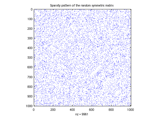
The command "eigs" finds only the few largest (or smallest) eigenvalues of a matrix. It uses an entirely different kind of algorithm; this algorithm is very well-suited to sparse matrices. Here, we'll demonstrate with a very large sparse matrix.
B = sprandsym(1000,.01);    % this is a 1000 x 1000 sparse symmetric matrix
                            % 1% of its entries are randomly selected to
                            % be nonzero; on those entries, the value is
                            % chosen from a uniform distribution.
spy(B); title('Sparsity pattern of the random symmetric matrix');
% Now, ask for the top and bottom 8 eigenvalues:
% (by "top", we mean those with the greatest magnitued; remember, the
% singular values may be complex)
opts = []; opts.disp = 0;  % tell the algorithm to be quiet!
opts.maxiter = 1500;       % tell the algorithm to be patient
disp('largest eigenvalues:')
D = eigs(B,8,'LM',opts)
disp('smallest eigenvalues:')
D = eigs(B,8,'SM',opts)

% Note: you can use this command to also get the eigenvectors, not just the
% eigenvalues
largest eigenvalues:

D =

    7.3641
   -7.1307
   -6.9764
    6.9301
    6.8860
   -6.8477
    6.7235
   -6.7186

smallest eigenvalues:

D =

    0.0207
    0.0149
    0.0030
   -0.0018
   -0.0073
   -0.0129
   -0.0181
   -0.0204
To see the biggest/smallest eigenvalues, in terms of the number and not the absolute value (this only works of eigenvalues are real, i.e. the matrix is symmetric), we use "LA" and "SA" instead of "LM" and "SM"
disp('largest eigenvalues:')
D = eigs(B,8,'LA',opts)
disp('smallest eigenvalues:')
D = eigs(B,8,'SA',opts)
largest eigenvalues:

D =

    7.3641
    6.9301
    6.8860
    6.7235
    6.6404
    6.5884
    6.5498
    6.5121

smallest eigenvalues:

D =

   -7.1307
   -6.9764
   -6.8477
   -6.7186
   -6.6361
   -6.5858
   -6.5508
   -6.5229
Singular Value Decomposition (SVD)
The SVD is vaguely like a a generalization of the eigenvalue decomposition; it gives slightly different information, and it is also more general (i.e. it applies to non-square matrices). We factor a matrix A as the product of three matrices: A = U * S * V'. S need not be square, but it is zero except on the diagonal. There are important variations, called the "thin" or "compact" svd. The diagonal entries of S are called the singular values, and they are always real and positive. By convention, they are always listed in decreasing order. In Matlab, the function to generate the SVD is called "svd()", and there is also a sparse version ("svds()"). Like "eig", we can ask for the singular values only, or the singular values and the singular vectors (the vectors refer to U and V).
clear; A = randn(5);
disp('The singular values of A are:')
s = svd(A)
disp('The singular values and singular vectors of A are:');
[U,S,V] = svd(A)
fprintf('Norm of A - U*S*V'' is %.3e\n', norm( A - U*S*V') )
The singular values of A are:

s =

    3.2378
    2.5077
    1.4542
    0.7395
    0.3905

The singular values and singular vectors of A are:

U =

    0.3517    0.1627   -0.1112    0.5941   -0.6961
   -0.0600    0.3884   -0.4855   -0.6567   -0.4225
    0.8330   -0.4254   -0.1979   -0.2638    0.1280
    0.1207   -0.0322    0.8235   -0.3800   -0.4024
    0.4052    0.8004    0.1862    0.0425    0.3983


S =

    3.2378         0         0         0         0
         0    2.5077         0         0         0
         0         0    1.4542         0         0
         0         0         0    0.7395         0
         0         0         0         0    0.3905


V =

    0.0228   -0.2760   -0.1907   -0.9390   -0.0720
    0.7186    0.6327    0.0598   -0.1630   -0.2304
   -0.5086    0.5408   -0.6232   -0.0260   -0.2446
   -0.2752    0.4663    0.3626   -0.2716    0.7082
   -0.3855    0.1168    0.6635   -0.1312   -0.6167

Norm of A - U*S*V' is 2.221e-15
The SVD is a robust method to determine the rank of a matrix. The rank is simply the number of nonzero singular values. In practice, there is a little difficulty because we may find tiny singular valies (1e-15) that are not quite zero; do these count or not? In general, Matlab will apply some thresholding (probably after normalizing by the largest singular value).
clear; T = randn(5,2);  A = T*T';  % A is a 5 x 5 matrix, with rank 2
disp('The singular values of A are:')
s = svd(A)
disp('The rank of A is:')
r = rank(A)
The singular values of A are:

s =

    3.8765
    1.5813
    0.0000
    0.0000
    0.0000

The rank of A is:

r =

     2
The sparse version, "svds", works very similarly to "eigs". It is not one of Matlab's finest algorithms, from a numerical analysis point-of-view. It simply calls "eigs" on a modified version of the matrix.
If you are interested in how the SVD or eigenvalue decomposition is performed, for the non-sparse case, Cleve Moler has a fantastic visual demonstration (for ACM 106, this is vey useful): http://www.mathworks.com/moler/ncm/eigsvdgui.m
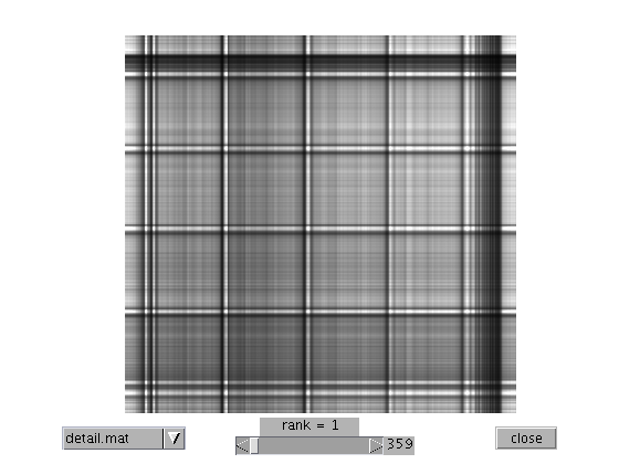
The SVD is a key ingredient in many techniques, such as Principal Component Analysis (PCA) and Latent Semantic Analysis (LSA). Cleve Moler's textbook includes a very nice routine that demonstrates the use of the SVD in approximating matrices (in this case, the matrices are pictures). This could lead to a good project... The following file can be found at: http://www.mathworks.com/moler/ncm/imagesvd.m
imagesvd
Numerical Integration, aka quadrature
Numerical integration is the process of approximating the value of an integral. We'll only cover definite integrals with finite endpoints, but it can be adapted for infinite endpoints. The general technique, called quadrature (not to be confused with other meanings of "quadrature"), is to sample the function f at a few points, interpolate these points piece-wise with a polynomial of degree n, integrate this polynomial exactly, and return this as our approximation. The interpolation and exact integration can be combined into one step, so no actual interpolation really happens. It is also not necessary to interpolate with a plain polynomial, but we will not cover this.
The simplest case is using polynomials of degree n = 0, i.e. use a piece-wise constant approximation. This is basically a Riemann sum. We can use linear polynomials to get the midpoint rule.
Matlab can do all this for us, and it will chose gridpoints adaptively. The workhorse routine is "quad()", but there are other variants (type "help funfun" and see the quadrature section). Simpler methods are "trapz" and using "sum". Here's an example:
f = @(x) exp(-x);   % this is the integrand
a = 0;              % The integral is from a to b
b = 3;
integralExact = 1 - exp(-3);
fprintf('Exact integral is %.4f\n', integralExact );
% Use a very basic method, with N points
for N = [50, 100, 200, 1000, 10000]
    RiemannSum = sum( f( linspace(a,b,N) ) ) *(b-a) / N;
    fprintf('Riemann sum, with N = %5d, gives %.4f\n',N,RiemannSum);
end
% Use another very basic method, with N points
for N = [50, 100, 200, 1000, 10000]
    trapRule = trapz( f( linspace(a,b,N) ) ) *(b-a) / N;
    fprintf('Trapezoidal Rule, with N = %5d, gives %.4f\n',N,trapRule);
end
% and use a smarter method:
[adaptiveSimpson,N] = quad(f,a,b);
fprintf('Using matlab''s "quad", with N = %d, gives %.4f\n',N,adaptiveSimpson);
Exact integral is 0.9502
Riemann sum, with N =    50, gives 0.9630
Riemann sum, with N =   100, gives 0.9565
Riemann sum, with N =   200, gives 0.9534
Riemann sum, with N =  1000, gives 0.9508
Riemann sum, with N = 10000, gives 0.9503
Trapezoidal Rule, with N =    50, gives 0.9315
Trapezoidal Rule, with N =   100, gives 0.9408
Trapezoidal Rule, with N =   200, gives 0.9455
Trapezoidal Rule, with N =  1000, gives 0.9493
Trapezoidal Rule, with N = 10000, gives 0.9501
Using matlab's "quad", with N = 25, gives 0.9502
dialog boxes, etc.
Matlab can popup dialog boxes (see "dialog" or "msgbox"). Here's an example of a waitbar -- it graphically displays a sliding counter.
h = waitbar(0,'Computing...');
for i = 1:300
    pause(.01);         % wait .01 seconds
    % (usually, a lengthy computation goes here)
    waitbar(i/300,h);
end
close(h);
For other length computations that update a graph at every step, use the command "drawnow" afer a "plot" command to force the graph to refresh, otherwise Matlab might wait to draw the graph until all the computation is done. For the most efficient way to update a graph, change the XData using handle graphics, or link the variables (see last lecture for how to do this).
"while" statement; "break"
The "while" statement is very similar to a "for" statement, and usually you can interchange the two (with appropriate modifications), but sometimes one or the other makes more sense. The idea is that the code is executed UNTIL some condition stops. The format is:
while [test] [body of code] end
and it will execute until the test if false. The simplest example is like a "for" loop:
clc;
j = 1;
while j < 10
    j = j + 1;
end
fprintf('j is now %d\n', j)
j is now 10
The example above doesn't take full advantage of a "while" statement. In general, the body of the code would something very complicated. Here's an example
seed = 0;
mn = 0;
while (mn < .6) && (seed < 10000)
    seed = seed + 1;
    rand('state',seed);
    mn = mean( rand(15,1) );
end
fprintf('Took %d tries to find a random vector with mean >= .6\n',seed);
Took 44 tries to find a random vector with mean >= .6
Here's how we can do the same using a "for" loop, with a "break" statement. Whenever a "break" statement is called, the most local "for" loop will quite.
for seed = 1:10000
    rand('state',seed);
    mn = mean( rand(15,1) );
    if mn >= .6
        break;
    end
	seed = seed + 1;
end
fprintf('Took %d tries to find a random vector with mean >= .6\n',seed);
Took 44 tries to find a random vector with mean >= .6
Dealing with errors
There are two things we'd like to do with errors: (1) when we write our own code, we might want to "throw" an error, and (2) when Matlab generates an error, we might want to do something special. First, let's cover (1). When we throw an error, execution will stop. The simplest way to throw an error is just using "error('message')"
% error('This is an error message')
We can also give an ID to the message (this is useful if some program is going to do something about the error):
% error('lectureNotes:ErrMsg1','Another error message')
For objective (2), here's how to see some information about an error. We use the function "lasterror" as follows:
errInfo = lasterror
% The "stack" field is itself a structure,and contains information about
% where the error occurred (e.g. which file, which function, and which
% line).  This doesn't work when the code was executed in "cell mode"!
errInfo =

       message: ''
    identifier: ''
         stack: [0x1 struct]
Also as a part of objectve (2), we can handle Matlab's errors using "try" and "catch". Here's how:
try
    size( thisVariableDoesNotExist );   % because the variable doesn't exist,
                                        % Matlab will generate an error.
catch
    % If an error is thrown, then the code here will be executed:
    errInfo = lasterror;
    fprintf('Message identifier is: %s\n',errInfo.identifier);
    fprintf('Message string is: %s\n',errInfo.message);
    % and if we want to le the error continue, we can "rethrow" it:
    rethrow( lasterror );
end
Error using ==> evalin
Undefined function or variable 'thisVariableDoesNotExist'.