ACM11 Homework 3 Solutions
Contents
Problem 1(a): Raptor ODE
There are different approaches to using the cutoff. Here are two different implementations.
Version 1: timeToDeath.html
Version 2: timeToDeath_2.html
and the caught.html file used in version 2.
Problem 1(b): Optimizing the angle
First question: what's the worst direction to run (or, from the raptor's perspective, the quickest way to a meal)? Intuitively, the answer is -30 degrees or -150/+210 degrees (i.e. running straight at either healthy raptor). However, due to inaccuracies in the ODE solver, we may not get -30 exactly. In research, this is not OK! But for this class, an answer between -20 and -40 (or -140 to -160) is acceptable. We can see that of the two methods implemented above, the second one is much quicker and more accurate.
tic; [ang,val,flg] = fminbnd(@timeToDeath,-180,180); t = toc;
fprintf('Using implementation 1, worst angle is %.2f and it took %5.2f s to calculate\n', ang, t);
tic; [ang,val,flg] = fminbnd(@timeToDeath_2,-180,180); t = toc;
fprintf('Using implementation 2, worst angle is %.2f and it took %5.2f s to calculate\n', ang, t);
Using implementation 1, worst angle is -35.27 and it took 57.90 s to calculate
Using implementation 2, worst angle is -30.88 and it took  3.41 s to calculate
Now, what's the best direction to run? If the injured raptor is really slow, then the best strategy is to run straight at it. But in our case, the best strategy is not obvious, so we resort to numerical methods.
tic; [ang,val,flg] = fminbnd(@(a)-timeToDeath(a),-180,180); t = toc;
fprintf('Using implementation 1, best angle is %.2f and it took %5.2f s to calculate\n', ang, t);
tic; [ang,val,flg] = fminbnd(@(a)-timeToDeath_2(a),-180,180); t = toc;
fprintf('Using implementation 2, best angle is %.2f and it took %5.2f s to calculate\n', ang, t);
Using implementation 1, best angle is 55.81 and it took 52.22 s to calculate
Using implementation 2, best angle is 54.55 and it took  3.30 s to calculate
Problem 1 BONUS
One bonus question was: if the injured raptor moves really slowly, then the optimal strategy is to run straight at it. So, at what speed for the injured raptor is it no longer optimal to run straight at it? The question is well-posed, because if the top raptor isn't injured, then clearly the optimal strategy is to run exactly in between any two of the raptors.
Even if you don't have an analytic solution, we can still find a precise answer using numerical methods. First, set the injured raptor's speed to 0, tell the human to run straight at the injured raptor (90 degrees) and calculate the time to death (the two healthy raptors should arrive at the same time). This comes out to about .5437 seconds. In .5437 seconds, the human has travelled 6*.5437 meters. The key insight is that the critical speed of the injured raptor is the speed at which all three raptors arrive at the human's location at the same time. So, the top raptor, who starts 20*sqrt(3)/3 meters above the human, has to travel 20*sqrt(3)/3 - 6*.5437 meters in .5437 seconds. This leads to a critical speed of about 15.2 m/s.
Actually, we ignored the .1 m radius around the human, but it doesn't matter: really, the human has travelled 6*.5437 + .1 meters, but the injured raptor actually has .1 m less to travel, so the .1 cancels.
Problem 2(a): Convolution
There are quite a few ways to implement this. Here's on method:
Let's check that it works by comparing to Matlab's "conv" function. We expect the error to be zero, or at least around machine precision (i.e. 1e-15).
a = randn(100,1); b = randn(90,1);
err = norm( convSlow(a,b) - conv(a,b) );
fprintf('Error is %.3e\n',err);
Error is 2.205e-14
Now, test the output
randn('state',2008);
f = randn(80000,1);
g = randn(40000,1);
tic; c = convSlow(f,g); t = toc;
fprintf('30th element is %.3f, and it took %.2f seconds \n', c(30),t );
30th element is 0.277, and it took 105.24 seconds
The speed of your program depends a lot on which version of Matlab you have (due to hidden optimizations), but also on how you structure the code. There are a few cases you have to deal with, and it is more efficient to put each case in its own "for" loop, rather than have one big "for" loop with an "if" statement inside. The "if" statement is rather slow; in general, the rule-of-thumb for "for" loops is to keep the body of the inner-most "for" loop as simple as possible.
Problem 2(b): Fast Convolution
See
convFast.html
A basic code pads the vectors with zeros so that both are length n1+n2-1 (where one vector is originally length n1, and the other length n2). For speedier code, it is sometimes useful to round this number to the nearest power of 2, because the FFT is very efficient for powers of 2. For old FFT code, this was almost always the case, but newer FFT code has made great strides in practical speed for non-powers-of-two. But in this case, rounding does seem to help. It also depends on how much rounding is required: rounding a vector of length 1025 (=2^10+1) to a power of 2 would lead to 2048 (we can't round down, or else we'd lose data), which is a lot of unneccesary computation. Highly composite numbers are generally faster than primes, although in theory, O(N*log(N)) algorithms exist for any number N, even primes.
Let's check that it works by comparing to Matlab's "conv" function. We expect the error to be zero, or at least around machine precision (i.e. 1e-15).
a = randn(100,1); b = randn(90,1);
err = norm( convFast(a,b) - conv(a,b) );
fprintf('Error is %.3e\n',err);
Error is 3.858e-14
Now, test the output. Note that our function is much faster than "conv"!
randn('state',2008);
f = randn(80000,1);
g = randn(40000,1);
tic; c = convFast(f,g); t = toc;
fprintf('30th element is %.3f, and it took %.2f seconds \n', c(30),t );
30th element is 0.277, and it took 0.05 seconds
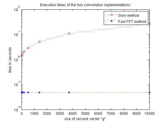
Problem 2(c): plotting the times
timesSlow = zeros(8,1);
timesFast = zeros(8,1);
nList = round(logspace(1,4,8));
for i = 1:8
    g = randn( nList(i), 1);
    tic; convSlow(f,g); t = toc;
    timesSlow(i) = t;
    tic; convFast(f,g); t = toc;
    timesFast(i) = t;
end
semilogy(nList,timesSlow,'ro:',nList,timesFast,'b*:');
title('Execution times of the two convolution implementations');
xlabel('size of second vector "g"');
ylabel('time in seconds');
legend('Slow method','Fast FFT method');