Lecture 2, ACM 11
Contents
- These lectures are online
- Review of matrix and vector norms (on blackboard)
- Review of Gaussian Elimination and condition numbers (on blackboard)
- Basic plotting
- More on matrices
- Pre-allocation
- Vectorization
- Logicals and "if" statements
- "if" statement is slow
- Find
- MATLAB uses finite precision
- "format" command
- Data types
- single precision
- Strings, and displaying messages
- fprintf, sprintf
- Useful commands for dealing with files
- saving variables the easy way
- anonymous functions
These lectures are online
see http://www.acm.caltech.edu/~acm11/2008/FALL/html/lecture1.html and http://www.acm.caltech.edu/~acm11/2008/FALL/html/lecture2.html
Review of matrix and vector norms (on blackboard)
key point for all norms: norm(x) = 0 if and only if x = 0
clc; x = randn(20,1); A = randn(20,20);
disp('Vector norms:')
disp(norm(x))         % if given no second argument, the default is "2"
disp(norm(x,2))
disp(norm(x,1))
disp(norm(x,'inf'))
disp('Matrix norms:')
disp(norm(A))         % if given no second argument, the default is "2"
disp(norm(A,2))
disp(norm(A,'fro'))
disp(norm(A(:)))      % A(:) puts the matrix A into a long vector
disp(' "inf" norms')
disp(norm(A,'inf'))
disp(norm(A(:),'inf'))  % these are NOT the same
disp('  "1" norms')
disp(norm(A,1))
disp(norm(A(:),1))      % these are NOT the same
Vector norms:
    4.2139

    4.2139

   15.7541

    1.7666

Matrix norms:
    7.8173

    7.8173

   19.8619

   19.8619

 "inf" norms
   19.1169

    3.0010

  "1" norms
   22.8393

  325.8085
Review of Gaussian Elimination and condition numbers (on blackboard)
lu factorization ("lu") is Gaussian Elimination. If the matrix is positive definite, use Cholesky factorization instead (Matlab function: "chol") If the matrix isn't square, or isn't full rank, the backslash operator will give the same result as using the pseudo-inverse ("pinv"). If the system is under-determined, there are infinitely many answers, and the backslash operator will return the "smallest" answer, in the sense of the l_2 norm. If the system is over-determined, there is probably no solution, so the backslash operator will return the vector that minimizes the residual.
% The condition number tells you a bit about how easy it is to solve a linear
% system on a computer.  Suppose we want to solve the equation Ax = b, and our
% matrix A looks like this:
clc;A = [1 4; 2 8];
% A is not invertible, so there is either no solution, or infinitely many
% solutions.
b = [894.4272; -447.2136];  % this is not in the range of A
x=A\b                         % so there is no solution
Warning: Matrix is singular to working precision.

x =

  -Inf
   Inf
But what if we change A just a bit?
A = [1 4; 2 8.0000000000001]
x=A\b
disp(['Residual is ', num2str( norm(A*x-b) )])
% the residual is rather large, for even a 2 x 2 system
% This is reflected in the fact that the condition number for the matrix A
% is large.  If A is singular, the condition number is (theoretically)
% infinite.
disp(['Condition number of A is ', num2str(cond(A)) ])
A =

    1.0000    4.0000
    2.0000    8.0000


x =

   1.0e+16 *

    8.9914
   -2.2478

Residual is 1.7584
Condition number of A is 823057853241041.6
Basic plotting
MATLAB plotting usually requires a list of points to plot (the exception "ezplot", which we discussed in the first lecture). This is
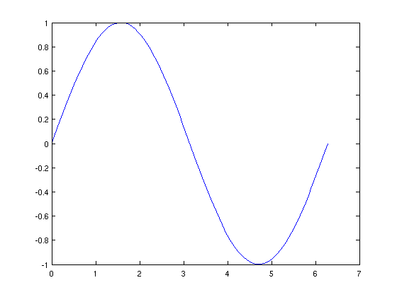
%different than Mathematica, or a TI calculator, and might take a while
%to get used to.  The basic plotting syntax is simple
clc;
X = linspace(0,2*pi,100);
Y = sin(X);
plot(X,Y)
% we can control colors, and markers (see "help plot" for all possible
% options)
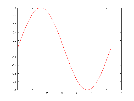
plot(X,Y,'r-')  % the "r" is for red, and the "-" tells MATLAB to draw a
                % solid line
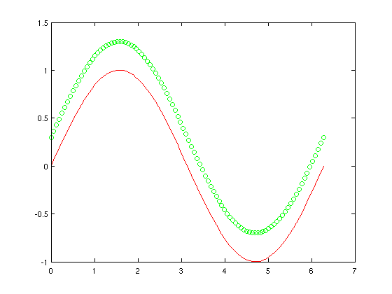
A few basic plotting tools: if we plot something new, the old plot will be destroyed, unless we type "hold on" AFTER the first plot.
hold on
plot(X,Y+.3,'go');  % the "g" is for green, the "o" tells MATLAB to draw
                    % little circles
We can put several plots in the same figure, using "subplot"
clf;        % clears the figure
subplot(1,2,1); plot(X,Y,'r-'); title('SUBPLOT 1');
subplot(1,2,2); plot(X,Y+.3,'go'); title('SUBPLOT 2');
% you can change axis limits and such.  For example, to make the x and y
% axis have the same spacing (useful for pictures), use:
axis square     % this ONLY affects the second subplot
xlabel(' x ');      % same would work for "y" too, of course
subplot(1,2,1);     % go back to the first plot
ylim( [-.5,.5] );

You can open several figures. Use the "figure" command. If you have a figure window that says "Figure 1", then the command "figure(1)" will make all the actions of any plotting go to that figure window. You can switch back and forth at will.
for 3D plotting, use "plot3". There are also many other 3D plotting tools (for contour plots, etc.). You can get a list of them by typing "help graph3d". Similarly, "help graph2d" gives normal 2D plots. There are some special functions (like a histogram, or a pie chart) that you can find in the listing "help specgraph". For images, "image" and "imagesc" are useful.
More on matrices
For more help, type "help matfun" and "help elmat". Basic matrix creation functions:
format; clc; Z = zeros(5,5)
% Note: zeros(5) is a shortcut for zeros(5,5)
O = ones(5,6)
I = eye(4,5)
% type "help gallery"
% for many example matrices
H = invhilb(5)
Z =

     0     0     0     0     0
     0     0     0     0     0
     0     0     0     0     0
     0     0     0     0     0
     0     0     0     0     0


O =

     1     1     1     1     1     1
     1     1     1     1     1     1
     1     1     1     1     1     1
     1     1     1     1     1     1
     1     1     1     1     1     1


I =

     1     0     0     0     0
     0     1     0     0     0
     0     0     1     0     0
     0     0     0     1     0


H =

          25        -300        1050       -1400         630
        -300        4800      -18900       26880      -12600
        1050      -18900       79380     -117600       56700
       -1400       26880     -117600      179200      -88200
         630      -12600       56700      -88200       44100
About indexing: you cannot create and then index a matrix in the same step!
H = invhilb(5);
h = H(3,4)
% h = invhilb(5)(3,4) would not work
h =

     -117600
Vectors and matrices can be changed dynamically! Very nice
clc; A = eye(5)
A = [A; A]      % we overwrite A with the expression
A =

     1     0     0     0     0
     0     1     0     0     0
     0     0     1     0     0
     0     0     0     1     0
     0     0     0     0     1


A =

     1     0     0     0     0
     0     1     0     0     0
     0     0     1     0     0
     0     0     0     1     0
     0     0     0     0     1
     1     0     0     0     0
     0     1     0     0     0
     0     0     1     0     0
     0     0     0     1     0
     0     0     0     0     1
Pre-allocation
We can change the size of matrices whenever. However, there is a cost. MATLAB needs to re-allocate RAM whenever this happens. To speed things up, we can allocate all the memory at once. For example, to create the Hilbert matrix:
clc; clear;
N = 1000;
tic
for i = 1:N
    for j = 1:N
        % make sure to use a semicolon to suppress output!
        % Otherwise, it'll take forever.
        A(i,j) = 1/(i+j-1);
    end
end
toc
Elapsed time is 11.562118 seconds.
Now, pre-allocate space for the matrix
tic
B = zeros(N);
for i = 1:N
    for j = 1:N
        B(i,j) = 1/(i+j-1);
    end
end
toc
Elapsed time is 2.698717 seconds.
And even faster, use MATLAB's own commands
tic; C = hilb(N); toc
Elapsed time is 0.080907 seconds.
Vectorization
Why was our code so much slower than MATLAB's code? We didn't take advantage of vector operations. But, we can fix that
N = 5;
d = 1:N;
Dx = repmat(d,N,1);     % "repmat" stands for Repeat Matrix
Dy = repmat(d',1,N);    % We make a new, bigger matrix out of copies
                        % of the smaller matrix
D = ( Dx + Dy - ones(N) ).^-1
hilb(5)                 % compare our code to make sure we are correct
D =

    1.0000    0.5000    0.3333    0.2500    0.2000
    0.5000    0.3333    0.2500    0.2000    0.1667
    0.3333    0.2500    0.2000    0.1667    0.1429
    0.2500    0.2000    0.1667    0.1429    0.1250
    0.2000    0.1667    0.1429    0.1250    0.1111


ans =

    1.0000    0.5000    0.3333    0.2500    0.2000
    0.5000    0.3333    0.2500    0.2000    0.1667
    0.3333    0.2500    0.2000    0.1667    0.1429
    0.2500    0.2000    0.1667    0.1429    0.1250
    0.2000    0.1667    0.1429    0.1250    0.1111
so, how fast is our new code?
N = 1000;
tic
d = 1:N;
Dx = repmat(d,N,1);
Dy = repmat(d',1,N);
D = ( Dx + Dy - ones(N) ).^-1;
toc
% it's fast!
Elapsed time is 0.136440 seconds.
Logicals and "if" statements
%{
    The "if" statement looks like:
if [test]
    [body]
end
    or there are more complicated forms, like:
if [test]
    [body]
elseif [test2]
    [body]
else
    [body]
end

the [test] will be evaluated as a logical
%}
% the simplest logicals are "true" and "false", e.g.
clc;clear; x = true
if x
    disp('x is true')
else
    disp('x is false')
end
x =

     1

x is true
a more compact form:
if false, disp('TRUE!'); else disp('FALSE!'); end
FALSE!
when we write "x = true", we could have written "x = 1" and had the same effect. However, there is a difference, because "true" is stored as a logical, which is one byte of memory, and "1" is stored as a floating point number, which is is 8 bytes of memory. We can see this with the command "whos", which displays workspace variables (the command "who" is similar, but doesn't tell you the size of variables). To make things confusing, if you type "true", MATLAB prints "1". But this is a logical 1, not a double 1. You can't tell the difference by looking at it, only with the "whos" command (or in the variable browser).
clear;x = 1;
y = true;
whos
  Name      Size                    Bytes  Class

  x         1x1                         8  double array
  y         1x1                         1  logical array

Grand total is 2 elements using 9 bytes
MATLAB will evaluate ANY nonzero number to "true".
clc
if .000001
    disp('true');
end
true
the [test] is often a comparison:
if   5 > 3
    disp('5 really is greater than 3');
end
% where the statement "5>3" is actually a logical.  For example,
myTestStatement = 5 > 3
% this command is setting myTestStatment as the result of the test (5>3).
% Other inequalities are <, >= and <=
5 really is greater than 3

myTestStatement =

     1
To do equality comparisons, make sure to use TWO "=" signs:
x = 5;
if x == 10
    disp('X is 10');
else
    disp('X is not 10');
end
% if you use a single "=" sign, the assigment is performed.  Hopefully,
% MATLAB will notice this and give you an error:
% if x = 10
%     disp('X is 10');
% else
%     disp('X is not 10');
% end

% For an inequality, use "~=", e.g.  if x ~= 10, ...
X is not 10
You can negate the outcome of a test, or of a logical, with "~". e.g.
clc
~true
~false
ans =

     0


ans =

     1
and you can double-negate something to turn it into a logical (you can also do this with the "logical" command).
clc; disp('Double negation:');
~~0
~~.0001
~~'d'
Double negation:

ans =

     0


ans =

     1


ans =

     1
all of this stuff is "vectorized":
~~[4 -3.2 pi 0 100]
% the vectorized command is very useful in conjunction with "find"
ans =

     1     1     1     0     1
Other useful tests:
% isequal, isreal, isnumeric, islogical, ischar, isfinite, isinf, isnan

% And the most powerful one is isa(...).  For example,
clc; x = true;
isa(x,'logical')
% See the "help" for isa.  You can check whether the variable is an
% integer, or a structure, or a cell, or a function, etc.
ans =

     1
Combining tests. In addition to negation ("~"), you can do "or" ("|") and "and" ("&"). These apply to entire vectors:
[true true] & [true false]
% You can also use "%%" and "||", but these must take scalar inputs.  The
% following will not work:
% [true true] && [true false]
% The only advantage to "&&" and "||" is that they only execute as much
% code as they have to (useful if the test itself takes a while to run).
% For example, in comparing "a && b", if "a" is false, then there is no
% need to evaluate "b", because the result of the test is already
% determined.
ans =

     1     0
Why is this useful? Here's an example
clc
test =  ~exist('myVariable') || myVariable <= 4 ;
% test =  ~exist('myVariable') | myVariable <= 4 ;  % fails!
if test
    disp('Either my variable doesn''t exist, or is 4 or smaller');
else
    disp('my variable is greather than 4');
end
Either my variable doesn't exist, or is 4 or smaller
Vector tests: "all" and "any"
clc
all( [true true false])
any( [true true false])
ans =

     0


ans =

     1
"if" statement is slow
e.g. we have to vectors x and y, and for each element x_i and y_i, we want to form a new element z_i where z_i is 2*x_i if x_i > y_i, and z_i is -y_i if x_i <= y_i.
clc; clear
N = 7;
y = randn(1,N)
x = randn(1,N)
% The plain way to create z:
for i = 1:N
    if x(i) > y(i)
        z(i) = 2*x(i);
    else
        z(i) = -y(i);
    end
end
z
disp('and the "MATLAB-way" to create z:');
z = 2*x.*( x > y ) - y .*( x <= y)
% much, much faster!
y =

   -0.9022   -0.5476    1.9871   -0.3817   -0.8528   -0.4826   -1.8569


x =

    1.1058    0.6375   -1.7107   -1.0510    0.9185   -0.7085   -0.2765


z =

    2.2116    1.2749   -1.9871    0.3817    1.8370    0.4826   -0.5529

and the "MATLAB-way" to create z:

z =

    2.2116    1.2749   -1.9871    0.3817    1.8370    0.4826   -0.5529
Let's repeat the previous command, but with bigger vectors so that we can see a difference in the time.
clc; clear
N = 50000;  % remember: to end execution of a program, type Ctrl + c
y = randn(1,N); x = randn(1,N);
tic
for i = 1:N
    if x(i) > y(i)
        z(i) = 2*x(i);
    else
        z(i) = -y(i);
    end
end
toc
disp('and the "MATLAB-way" to create z:');
tic;
z = 2*x.*( x > y ) - y .*( x <= y);
toc
Elapsed time is 12.634532 seconds.
and the "MATLAB-way" to create z:
Elapsed time is 0.007187 seconds.
Find
using "find"
clc; clear; H = abs(invhilb(5))
f=find( H < 1000 )  % this uses linear indexing
% find returns a list of indices, NOT of values of the matrix
H =

          25         300        1050        1400         630
         300        4800       18900       26880       12600
        1050       18900       79380      117600       56700
        1400       26880      117600      179200       88200
         630       12600       56700       88200       44100


f =

     1
     2
     5
     6
    21
this is the command to find the values of the matrix that were found
H(f)
ans =

    25
   300
   630
   300
   630
We do operations on these entries, without affecting other entries
H(f) = 0 % it's statements like this that make MATLAB so powerful
H =

           0           0        1050        1400           0
           0        4800       18900       26880       12600
        1050       18900       79380      117600       56700
        1400       26880      117600      179200       88200
           0       12600       56700       88200       44100
clc; H
[I,J] = find( H );  % this time, using subscript indexing
                    % This is the same as find( H ~= 0 )
[I,J]
H =

           0           0        1050        1400           0
           0        4800       18900       26880       12600
        1050       18900       79380      117600       56700
        1400       26880      117600      179200       88200
           0       12600       56700       88200       44100


ans =

     3     1
     4     1
     2     2
     3     2
     4     2
     5     2
     1     3
     2     3
     3     3
     4     3
     5     3
     1     4
     2     4
     3     4
     4     4
     5     4
     2     5
     3     5
     4     5
     5     5
we can combine a few steps
H( H > 0 ) = -3;
H
H =

     0     0    -3    -3     0
     0    -3    -3    -3    -3
    -3    -3    -3    -3    -3
    -3    -3    -3    -3    -3
     0    -3    -3    -3    -3
MATLAB uses finite precision
Same as all computer languages EXCEPT symbolic math programs. First, observe that we can use scientific notation
clc; x = 10^-16
% or, more compactly,
x = 1e-16
format long
x
format short
x =

   1.0000e-16


x =

   1.0000e-16


x =

     1.000000000000000e-16
now, explain the following:
clc
1 + x - 1
%
x
ans =

     0


x =

   1.0000e-16
"format" command
Changes the DISPLAYED value only; it does not change the internal precision.
clc;x = 84.1471;
format short; x
format long; x
format short e; x
format long e; x
format rat; x
% Warning: the "rat" format (for "rational") is only an approximation
% The answer is probably NOT a nice fraction
format short;   % back to our default
x =

   84.1471


x =

  84.14709999999999


x =

   8.4147e+01


x =

     8.414709999999999e+01


x =

    2861/34
Data types
The default data type for a number in MATLAB is double precision floating point, usually just called a "double". This uses 64 bits (e.g. 8 bytes), and it basically stores a number in scientific notation. Because of the bit-limitation, there are some numbers that are too large and too small to store. We can find out what this range is:
clc; realmax
realmin
% The range is large!  For example, one estimate for the radius of the
% universe is 10^26 meters.  The radius of a proton is about 10^-15 meters,
% and the Planck Length is about 10^-25 meters.
% However, we still get problems easily.  Perhaps more important than the
% range is the machine epsilon.  This number is given in MATLAB by
eps
% A 'double' only has roughly 16 digits of precision.  This means that a
% number like
%   1.000000000000000000
% and
%   1.000000000000000001
% are the same to a computer.
% So, be careful!
ans =

  1.7977e+308


ans =

  2.2251e-308


ans =

   2.2204e-16
single precision
A single precision variable, also known simply as a "float", only uses 32 bits to store a number, offering about 8 digits of accuracy. If you want a single precision variable, you must tell MATLAB explicitly
clc;format long
pi
single(pi)
format short
% Why use single precision?  It takes up less RAM, which can help for huge
% calculations.  But in general, don't use single precision.  On most
% modern computers, it probably won't make calculations faster; in fact, it
% in MATLAB, it will probably make everything slower (note: this may not be
% true in C or Fortran).
ans =

   3.14159265358979


ans =

   3.1415927
Strings, and displaying messages
clc;
num2str( 8 )    % converts a number to a character;
                % see also "int2str"
% the "disp" function requires a string input; you can paste several
% strings together.  But, if you have several strings, make it into a
% matrix.  For example, the following works:
disp(['The best even number is ' num2str(8) ]);
% but the following doesn't work:
%    disp('The best even number is ' num2str(8) );

% if you're dorky, you can do this:
disp(  strcat('The best even number is ',num2str(8) )   );
% but it took away the extra whitespace!
ans =

8

The best even number is 8
The best even number is8
for example, to find the current time
year = datestr(now,'yyyy');     % get the current year
disp( ['The current year is ', num2str(year), ' A.D.' ] );
The current year is 2008 A.D.
fprintf, sprintf
This is another way to print stuff to the screen
time = datestr(now,14);     % get the time (this is a string)
fprintf('The time is: %s\n', time)
% this command is much more powerful than "disp", but more complicated.
% We'll only go over a few features.  The "%s" is a placeholder for a
% string.  Common place holders are:
%   %d      for integer
%   %f      for float (either single or double)
%   %e      for scientific notation
% most of these take additional options, like
%   %.6f    will print the number with 6 decimal places.
% There are also special characters, like \t for tab andn \n for newline
%
% So, here are some examples
clc
fprintf('The %02d %s each ate %d bowls of \nporridge before devouring %s\n\n',...
    3,'bears', 19, 'a very tasty Goldilocks');
% the "%02d" requests 2 digits, and the 0 tells MATLAB to use a 0, not a
% space, if not all 2 digits are needed (so it displays 03 instead of  03).
fprintf('As a Caltech student, I can recite pi to 16 digits: %.16f\n',pi)
fprintf('And as a starving grad student, I can eat about %.2e pies\n', 150);
The time is:  5:29:19 PM
The 03 bears each ate 19 bowls of
porridge before devouring a very tasty Goldilocks

As a Caltech student, I can recite pi to 16 digits: 3.1415926535897931
And as a starving grad student, I can eat about 1.50e+02 pies
sprintf( ) is similar to fprintf, but just creates a string and doesn't display it.
s = sprintf('HELP! I AM TRAPPED INSIDE A COMPUTER!');
disp(s)
% This might be useful if you want to load many files.  You make the
% filename using sprintf, and then pass this string into the "load"
% function (or "fopen" -- see below)
HELP! I AM TRAPPED INSIDE A COMPUTER!
To use a ' inside a quote, write ''. This works for "disp" and "fprintf"
disp('Dave: Open the pod bay doors, HAL.');
disp('HAL: I''m sorry Dave, I''m afraid I can''t do that.');
Dave: Open the pod bay doors, HAL.
HAL: I'm sorry Dave, I'm afraid I can't do that.
fprintf can be used to print to a file. Here's how:
fileID = fopen('testFile.m','w');
if fileID == -1
    disp('uh oh');
else
    fprintf(fileID,'\n\n*** testing ***\n');
    fclose( fileID );
end
Useful commands for dealing with files
% "edit" allows you to open a file in the MATLAB editor
edit testFile.m
% "edit" is another example of a command that can take either "command"
% mode input or "function" input.  In "command" mode, the input is either a
% string, or will be converted to one.  In "function" mode, it should be a
% variable.  For example:

% edit 'testFile.m'       % "command" mode again
% edit('testFile.m')      % "function" mode
% % which is the same as
% myString = 'testFile.m';
% edit(myString)          % "function" mode
% % but this will not work:
% edit(testFile.m)        % WRONG mode
this "edit" command is super-awesome. Observe:
edit randperm
edit minres
We can see MATLAB's internal code! This is very, very useful. It should also teach you good programming habits. But, it doesn't work for all functions
edit randn
edit fft
% These functions are "builtin", and are also highly optimized.
More commands:
clc
what        % displays MATLAB-related files in this directory
% "cd" will change your current directory
M-files in the current directory /home/srbecker/TA

hw1             lecture1        lecture3        testFile
hw1solutions    lecture2        problem1

MAT-files in the current directory /home/srbecker/TA

hw1data1      myFile
which fft % will tell you where the file resides in your filesystem
built-in (/opt/matlab/toolbox/matlab/datafun/@logical/fft) % logical method
You can run operating-system commands in several ways. The simplest way is with a "!"
clc
if ispc         % tests for Windows
    !dir
elseif isunix   % tests for unix/linux
    !ls
end
% Macintosh is just not cool enough to have its own command.  But, you can
% use the "computer" command.

% you can also use the "system" command, as well as "dos" and "unix"
% commands.
ACM104_0607	     headerSimple.tex  hw2.log			  matrixMult
ACM104_0708	     header.tex        hw2.out			  Moler
ACM105_0607	     html	       hw2.pdf			  Moler_mFiles
ACM105_0708	     hw1data1.mat      hw2.tex			  myFile.mat
ACM11_0708	     hw1.m	       hwTopics			  my_notes
acm11_ideas.txt      hw1.pdf	       installation_problems.txt  problem1.m
ACM11_outline.docx   hw1solutions.m    lecture1.m		  syllabus
ACM95c		     hw1.tex	       lecture2.m		  testFile.m
BeckerS_29955.pdf    hw1_v2.pdf        lecture2.m~		  textbooks.htm
cleanup.sh	     hw1_v2.tex        lecture3.m		  vim-tex_shortcuts.pdf
headerShortcuts.tex  hw2.aux	       lecture3.m~		  vim-tex_shortcuts.tex
saving variables the easy way
Use MATLAB's "save" and "load" commands. You can call these in two modes:
clc;
variable1 = pi;
variable2 = [5,6,7];
% save myFile variable1 variable2         % "mode 1"
save('myFile','variable1','variable2')  % "mode 2"

% Suppose we lost the variables:
clear
who         % this shows any variables
Then, to reload them, use "load", in one of the same ways
load myFile             % loads all availabe variables
load myFile variable1   % loads only variable 1
who
Your variables are:

variable1  variable2
anonymous functions
These are fantastically useful. You can use them like any MATLAB function, although they are a bit more limited. The syntax is as follows
% SYNTAX:
% nameOfFunction = @(x1,x2,...) [expression involving x1, x2, ...]

% Ex.
clc; frequency = 2;
mySine = @(x) sin( frequency * x )
mySine( [1, 5, 9] )
% the value for "frequency" has been FROZEN!  It will NEVER change.
frequency = 200000;  % This won't affect "mySine"
mySine( [1, 5, 9] )  % Same output as before
mySine =

    @(x) sin( frequency * x )


ans =

    0.9093   -0.5440   -0.7510


ans =

    0.9093   -0.5440   -0.7510
You do not have to use all of the listed inputs:
myFunction = @(x,y) x.^2 ;
myFunction( [1,5,9] )
ans =

     1    25    81
If you expect vector inputs, make sure the function behaves how you want
myFunction = @(x,y) x^2;        % this is BAD if you have a vector input
% myFunction( [1,5,9] )     % would produce an error
Other useful ways to use anonymous functions:
actual = 9;
myFunc = @(guess) fprintf('The error is %.3f\n', norm(actual-guess) );
myFunc( 3 )
The error is 6.000
Use it to make default arguments
complicatedFunction = @(a,b,c,d,e) a.^2 - b/2 + exp(c)./(d.^2+e.^2);

b = 2; c = 4; d = pi; e = 4.5;
% all values except "x" are now "frozen" in to "simpleFunction":
simpleFunction = @(x) complicatedFunction(x,b,c,d,e);
simpleFunction(4)
ans =

   16.8127
this works on MATLAB's functions too
clc;
A = randn(2);
f = @sum;   % The "@" let's MATLAB know that "sum" is a function and not
            % the name of a variable.
            % We could have also written f = @(x) sum(x);
f(A)        % This is the same as using "sum(A)"
% Now, suppose we wanted to sum along a different dimension:
f = @(x) sum(x,2)
f(A)

% Why is this so useful?  If you use the function "f" many times in your
% code, but later you want to change a parameter, now you only need to
% change it in one place.  It can also simplify code, and help you spot
% errors.
ans =

    0.8522    0.6582


f =

    @(x) sum(x,2)


ans =

   -0.1756
    1.6861