Lecture 3, ACM 11

Review of Matrices
Structures
Dynamic field names of structures
Arrays of structures, and structures of arrays
Cells
Functions
Documentation
Path
Global variables
switch statements
funfun
Minimization/Maximization, Optimization
ODEs
a stiff ODE
Plotting, part II
FFT (Fast Fourier Transform)
Making a plot with error bars

Review of Matrices

We'll need to discuss eigenvalues, so first a quick review of matrices. This is on the blackboard, so for a reference, see MathWorld or Wikipedia. Topics: diagonalizable, normal, jordan canonical form orthogonal/unitary, symmetric/hermitian matrices. Are eigendecompositions unique (or, when are they unique, and in what sense?)? Schur form, SVD

Structures

Structures are a datatype, and are very useful for organizing several variables, especially in conjunction with arrays. We'll start with the easiest use of a structure, where we have a single variable (no arrays). The distinguishing feature of a structure is that it can have "fields", and as many fields as you wish. To make a variable a structure, you can use the "struct" command, but this is usually not necessary. If a variable doesn't yet exist (or is set to something like an empty matrix), then just referring to a field will tell Matlab to make the structure for you. Access fields is done with the "." mark. For example,

clc; clear;
myStructure.month = 'October';  % this will create the variable "myStructure"
myStructure.day = 13;           % we create a new field
% The fields can represent have different datatypes
% If we display myStructure, this is what we see:
myStructure
% Or we can see just a particular field:
fprintf('The current month is %s\n', myStructure.month )
% There are some useful commands associated with structures.  To see them,
% see the "see also" section after running the "help struct" command.  In
% particular, we can use "fieldnames" to see a list of fields in the
% struct.  For much more information, in the Help browser (the graphical
% one), in the "Contents" tab, select "Matlab >> Programming Fundaments >>
% Built-In Classes (datatypes) >> Structures".

myStructure = 
    month: 'October'
      day: 13
The current month is October

Dynamic field names of structures

Suppose we have many fields, and want to access them all in an automated fashion. In the example below, we'll make a "structure of structures" (an alternative would be to make a "cell" of structures, or to use structures in combination with array).

clc; clear;
% Make a smaller level structure
experiment.date = 'Tuesday, October 13';
experiment.hypothesis = 'Undergraduates need 2 hours of sleep per night';
experiment.conclusion = true;

% Make a higher level structure
sociologyClass.experiment1 = experiment;

% Now, suppose we wish to add many experiments
for n= 2:8
    fieldName = sprintf('experiment%d',n);
    sociologyClass.(fieldName) = [];       % we don't yet have data
end

% We used the format   sociologyClass.(fieldName), and NOT the format
%                      sociologyClass.fieldName
% The parenthesis tell Matlab that we want to access the value of the
% variable inside "fieldName", and that the field is not actually called
% "fieldName".
sociologyClass

sociologyClass = 
    experiment1: [1x1 struct]
    experiment2: []
    experiment3: []
    experiment4: []
    experiment5: []
    experiment6: []
    experiment7: []
    experiment8: []

Arrays of structures, and structures of arrays

The usage of "structures of structures" is very versatile, and the low-level structures need not look identical (i.e. they can have different fields). If all the low-level structures are identical, then we can use an array. There are two options: an array of structs, and a struct of arrays.

clc; clear;
% === A struct of arrays ===
structArray.dayOfMonth(1) = 15;
structArray.dayOfMonth(2) = 7;
structArray.dayOfMonth(3:5) = [6, 5, 20];
structArray.digitsOfPi(1:7) = [3 1 4 1 5 9 6];
structArray.name(1,:) = 'Bob';
structArray.name(2,:) = 'Sam';
% structArray.name(2,:) = 'Nancy';  % would not work, because
                                    % Nancy is a different length than Bob
structArray

% === An array of structs ===
arrayStruct(1).dayOfMonth = 15;
arrayStruct(2).dayOfMonth = 7;
% arrayStruct(3:5).dayOfMonth = [6, 5, 20];   this does not work!
arrayStruct(5).dayOfMonth = 20;

arrayStruct(1).name = 'Bob';
arrayStruct(2).name = 'Nancy';
arrayStruct

structArray = 
    dayOfMonth: [15 7 6 5 20]
    digitsOfPi: [3 1 4 1 5 9 6]
          name: [2x3 char]
arrayStruct = 
1x5 struct array with fields:
    dayOfMonth
    name

Note that we actually have 5 spots allocated for the "name" field in arrayStruct, since we referenced the 5th element in referring to "dayOfMonth".

arrayStruct.name

ans =
Bob
ans =
Nancy
ans =
     []
ans =
     []
ans =
     []

So, which is better, an array of structs, or a struct of arrays? Both can be useful. For small amounts of data, use either. For large amounts of data, a struct of arrays is preferred, because this makes one structure and many arrays, and an array is a more "efficient" datatype than structure (however, this overhead can be irrelevant if the value of the field takes up a lot of memory). An array of structures makes many structures, and is more inefficient. For example,

clc; clear;
for j=1:40000
    structArray.field(j) = pi;
    arrayStruct(j).field = pi;
end

To see how big these variables are, we again use stuctures!

w = whos('structArray','arrayStruct')
% the "whos" command returns an array of structs, with fields like "name",
% "size", and "bytes".
for j = 1:length(w)
    fprintf('Variable %s takes up %.3f MB of RAM\n', w(j).name, w(j).bytes/(1024^2) );
end

w = 
2x1 struct array with fields:
    name
    size
    bytes
    class
    global
    sparse
    complex
    nesting
    persistent
Variable arrayStruct takes up 2.594 MB of RAM
Variable structArray takes up 0.305 MB of RAM

Cells

Cells are another Matlab datatype. A cell is like an array, except that every element of an array must be the same datatype (e.g. a character, or a double). Cells are not restricted like this. In syntax, the difference is that we use { and }; these curly braces are used for both creating and access elements of a cell (whereas for arrays, we have separate notation for both these). For example,

clc; clear
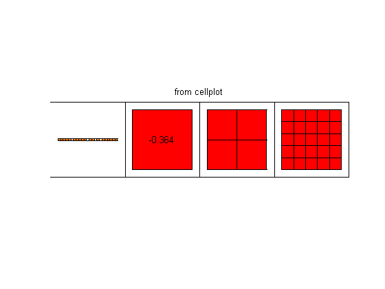
myCell = {'First entry is a string', -.364, [1 2; 3 4], ones(5) }
% Like structures, you can explicitly create a cell (use the command
% "cell"), but this is rarely necessary.

% This is a useful way to visualize the contents of a cell"
clf; cellplot(myCell); title('from cellplot');

myCell = 
    [1x23 char]    [-0.3640]    [2x2 double]    [5x5 double]

There are numerous functions for converting between datatpes (e.g. "cell2mat"), especially between strings and cells. Cells are a useful way to store strings (which are 1-D arrays of characters), because storing a 2-D array of characters requires you to pad short strings with zeros to make everything line up. Note that both cells and structs can be nested and intermixed.

For much more information on cells, in the Help browser (the graphical one), in the "Contents" tab, select "Matlab >> Programming Fundaments >> Built-In Classes (datatypes) >> Cell Arrays".

A word of caution: it is possible to use ( ) to access cell indices, but this doesn't do what you might think: instead of getting the element inside the cell, you actually get a single cell containg the element.

myCell = {'This is a string','Ceci n''est pas une corde' };

% To demonstrate, let's call the "deblankl" funuction, which is just a
% random Matlab function that operates on strings (it takes away whitespace
% and makes everything lowercase):
 disp( deblankl( myCell{1} ) );       % this is fine
%disp( deblankl( myCell(1) ) );       % this will give an error message

disp(myCell{1})     % with the curly brackets, we get a string
disp(myCell(1))     % with parenthesis, we get a new cell containing a string

thisisastring
This is a string
    'This is a string'

Functions

%{
    Functions are different than scripts.  They take a specified input
(usually), and give an ouput (usually), or perhaps print to the screen.  In
general, most functions don't have "side-effects".  This means that, if
you disregard their output, then calling the function won't affect the rest
of the code.  But, this is not always true, and not always desired; we'll
see this effect when we use "global" variables.  As an example, the function
"tic" has global effect.
    A function is defined in a separate file (unlike the anonymous
functions that we saw last lecture), and this file should have the same
name as the function (although not always required).  The syntaxt is:

function output = functionName( input )
[code...]

or, for several inputs/outputs:

function [output1, output2] = functionName( inputA, inputB)
[code...]

In the rest of the function body, all the variables that weren't passed
as inputs are "local".  This means they are completely different variables
than variables of the same name elsewhere.

There is no need to "end" the function, but you can if you wish; to do this,
just type "end" at the very end.  You do not need to have inputs or outputs,
so a line like:

function functionName

is valid.

Functions can have "sub-functions".  These are available ONLY to the main
function, and not to any other part of MATLAB.   To make a sub-function,
below the rest of the function code just use the same function syntax.  You
can make as many subfunctions as you want.  Again, there is no need to "end"
a subfunction, because Matlab can determine this automatically; but, if you do,
use the "end" keyword.  If you do this once in the function, you must do it
for all subfunctions.

One major advantage to Matlab is its flexibility in dealing with different
inputs and outputs.  You do not always need to pass all the arguments into
a Matlab function, and you do not always need to read out all possible output
values.  Inside the function, you can see how many parameters were passed
in with the "nargin" command (it returns an integer), and the number of
output variables is returned by the "nargout" command.  These are useful
for setting default values of parameters.

Another way to handle default arguments is by using structures.  The
disadvantage of "nargin" is that if we define a function like

function out = functionName( inA, inB, inC, inD)

and want to pass in values for "inA" and "inD", while using defaults
for "inB" and "inC", then we still need to give values to "inB" and "inC"
(otherwise "inD" will be interpreted as "inB").  Usually, we assign a
value like [ ] (the empty matrix), and check for this in the body of
the code using an "isempty" test.  But this is inelegant.  Structures can
be used to avoid this.  For example,

function output = functionName( essentialInput, options )
if ~isfield(options,'tolerance'), options.tolerance = 1e-6; end
...

If a certain option isn't set, then we gracefully set it to a default
value.

%}

Examples: to see subfunctions (and use of nargin and nargout), type "edit fzero". To see many more examples, just edit your favorite Matlab function. Many of the numerical functions show their source code (whereas functions that do low-level operations, such as loading a file, will not generally show the source code).

Documentation

In addition to adding comments to your code, there is a special section that is very useful. After the "function output = functionName(input)" line, the following commented lines are the "help" for that function. If you type "help functionName", it will show every comment that is written below the first line, until the first non-comment line (which includes any blank line). This is very useful! Use this, especially if someone else will need to use your code.

Path

When you type the name of a function, Matlab needs to know where to search for it. It can't search the entire hard drive, so it restricts itself to directories in the "path". To see which directories are in your path, just type "path", although you're likely to get more output than you want. There are many functions relating to the path. The most useful are "addpath", which adds a certain path to the directory, and "pathtool", which is a graphical tool that lets you manipulate the path. The current directory is always in the path. For any directory in the path, if it has a a subdirectory called "private", then the files in this subdirectory are also available, but only to files in the parent directory. This allows you to have many functions with the same name, but in different directories, without getting mixed up.

To see where a function resides, use the "which" command.

For example, if I want to use a Preconditioned Conjugate Gradient solver (this is a solver for huge linear systems), I can use Matlab's "pcg" function. This resides in C:\Program Files\MATLAB\R2008a\toolbox\matlab\sparfun

which pcg
if ispc
    winopen('C:\Program Files\MATLAB\R2008a\toolbox\matlab\sparfun')
end
% We see that there is a subdirectory called "private", which contains
% functions like "interapp.m".  This file, "interapp", is only available to
% functions in the "sparfun" directory (such as pcg).  I cannot see it!
which interapp
% "which" is also useful if you have several files with the same name.
% Matlab will call the first one it finds -- in other words, the *order* of
% directores in the path is important!  Use the "-all" flag for "which" to
% see all functions with the same name (e.g. "which -all times" will show
% all the different functions called "times"; we say that this function is
% "overloaded", meaning that there a different function is called depending
% on the type of input).

C:\Program Files\MATLAB\R2008a\toolbox\matlab\sparfun\pcg.m
'interapp' not found.

Global variables

Global variables are variables that can be accessed anywhere. However, before a function can access a global variable, it must declare it. And to change the value of a global variable in the main workspace, you also must declare the variable. To declare a variable, use the form:

global myGlobalVariable1 myGlobalVariable2
% (do NOT separate these with commas!)

% for examples, type "doc global".  When you "clear" variables,
% global variables are unaffected unless you type "clear global"
% or "clear all".  (Note: a useful command, similar to "clear", is "close",
% and is used to close figure windows; "close all" closes all figure
% windows).

On a related note, there are several "workspaces". This is mainly for advanced use of Matlab, so isn't very important. To use this feature, the functions "evalin" and "assignin" are useful. If, for example, you want to evaluate the "whos" command to get a list of variables in the main workspace, but you call "whos" from a function, then you can't see the main workspace variables unless you tell Matlab to use the correct workspace (via the "evalin" command).

switch statements

Used to simplify "if" and "elseif" statements. See the help documentation:

doc switch

 Overloaded functions or methods (ones with the same name in other directories)
   <a href="matlab:doc simulink/switch">doc simulink/switch</a>

funfun

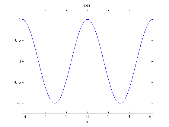
Can a function take another function as an input? Yes! We did it last week using anonymous functions. If we want to use a normal function, we can pass the function as an argument using a "function handle". Recall our "ezplot" example from lecture 1. This can accept a function handle, and use the function to plot. To get the "handle" to a funuction, just type "@" before the function name. Simple!

clf; ezplot( @cos )
% To see the most common Matlab functions that operate on other functions,
% type "help funfun".  These include functions that will find the minimum
% of other functions, as well as ODE solvers.
%
% To evaluate a function handle, usually you can treat it like a function.
% For example,
f = @cos;
f(pi)
% Sometimes you want to use "feval" (this is more robust; it accepts not
% only function handles, but strings with the name of a fuction).  The
% syntax is:
feval(f,pi)

ans =
    -1
ans =
    -1

Minimization/Maximization, Optimization

We are not going to cover the optimization toolbox. The conventional wisdom is that Matlab is very good at numerical linear algebra and related operations, but is relatively poor at optimization. But there are many excellent 3rd party Matlab applications, some of them free, that do optimization very well. A particularly simple package that I recommend is "cvx" by Michael Grant and Stephen Boyd.

For minimizing nonlinear functions, we can classify the algorithms according to how much information we have about the function. Do we know the derivative? Do we know the second derivative?

The basic functions for this in Matlab are "fminbnd", "fminsearch" and "fzero". If you have the optimization toolbox, then "fsolve" is another useful function. These do not require the derivative.

Most of these functions use structures to pass in additional arguments, as mentioned above.

% Example:
% What's the minimum of cosine, in the range 0 to pi?
clear;clc;
opts.TolX = 1e-2;
xmin = fminbnd( @cos, 0, pi, opts );
fprintf('Using a tolerance of %.2e, error is %.3e\n', opts.TolX, xmin - pi);
opts.TolX = 1e-9;
xmin = fminbnd( @cos, 0, pi, opts );
fprintf('Using a tolerance of %.2e, error is %.3e\n', opts.TolX, xmin - pi);

Using a tolerance of 1.00e-002, error is -6.030e-003
Using a tolerance of 1.00e-009, error is -9.410e-008

If you have the derivative information, and it's not computational expensive to compute the derivative at a point, then a good starting point is Newton's Method. This basically forms a linear model of your function, and finds the exact minimum of the linear model every step.

Be careful: Newton's Method sometimes refers to minimization, and sometimes to root-finding. The are related, since minimization of f is the same as finding a root of the derivative of f (if f has continuous derivatives). For root-finding, Newton's method needs a derivative; for minimization, it actually needs a second-derivative.

ODEs

%{
    ODE stands for Ordinary Differential Equation.  These differential
equations can involve several variables (often, we think of a single variable,
but allow it to be a vector).  They also involve derivatives of this vector
variable (say, x) with respect to a new variable (say, t).  Example:

x'' + 3*x' + t*x = -t + 9

where x' means d/dt (x).

    Types of ODEs: autonomous, linear, homogenous, constant-coefficient.
Note that all ODEs with higher derivatives can be turned into systems
of more variables, but only with first derivatives (for example, if we have
x'' = 3, we turn this into:
y' = 3;
x' = y;

    Basic ODEs can be solved with the matrix exponential.  To solve
the matrix exponential, you may have learned to diagonalze the matrix.
This is works well if, for example, if the matrix is symmetric, and we want
to find the value at many time points.  But if we only need a single time
point, there are much better ways to do it in practice for an arbitrary matrix.
For a general matrix, use Matlab's "expm" function.

    For tough ODEs that are not so simple, we can approximate the solution
with numerical methods.  The standard Matlab solver is "ode45".  Type
"doc ode45" for lots of good info.  To learn more about the algorithms,
take ACM106.
%}

a stiff ODE

This is perhaps the simplest possible example of a stiff ODE. In this example, the two variables decouple, so there is no reason to solve for them together (we could add a week coupling, although the solution wouldn't be as simple). But, suppose we solve for both variables at the same time. Because the two variables (y_1 and y_2) live on such different time scales, the standard solver ODE45 is confused, and solves for both variables on the small time scale. This requires very many time steps (since we have to run it for a long time -- due to the variable on the long time scale).

alpha = 1;
beta = 100000;
f = @(t,y) [-alpha*y(1); -beta*y(2)];
tic; [T,Y] = ode45(f,[0,1],[1;1] ); toc
tic; [Ts,Ys] = ode15s(f,[0,1],[1;1] ); toc
fprintf('Number of time samples used in ODE45:  %d\n', length(T) );
fprintf('Number of time samples used in ODE15s: %d\n', length(Ts) );
fprintf('l_infinity error via ODE45:  %.2e %.2e\n',...
    norm( Y(:,1) - exp(-alpha*T),'inf'), norm( Y(:,2) - exp(-beta*T),'inf') )
fprintf('l_infinity error via ODE15s: %.2e %.2e\n',...
    norm( Ys(:,1) - exp(-alpha*Ts),'inf'), norm( Ys(:,2) - exp(-beta*Ts),'inf') )
% We find that the "ode15s" solver is much better at handling the different
% scales than the "ode45" solver is.  "doc ode45" explains when to use the
% different solvers.

Elapsed time is 18.637057 seconds.
Elapsed time is 0.164729 seconds.
Number of time samples used in ODE45:  120573
Number of time samples used in ODE15s: 90
l_infinity error via ODE45:  2.50e-014 2.93e-004
l_infinity error via ODE15s: 1.92e-004 1.10e-003

Plotting, part II

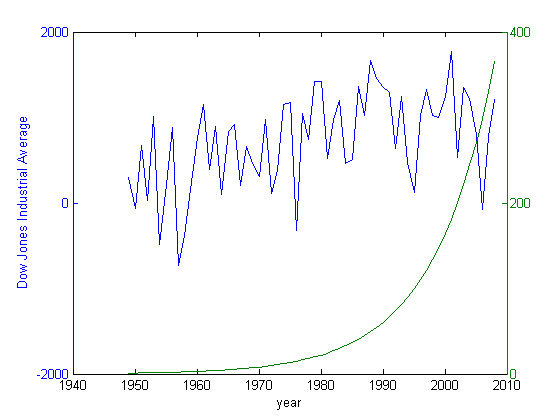
A common scenario for plotting is wanting to combine two variables on one plot, but have different scales for both of them. Matlab provides the "plotyy" command for this, and it will also give us a chance to see "handle graphics" for the first time. Handles are a tool that Matlab uses to identify objects. We've already seen handles when we used "fopen" and when we used function handles.

clear;clc; clf
% Example of two variables with different scales
t = 1949:2008;
stockMarket = 500*(randn(60,1)' + .05*(t-1949));
population = exp( .1*(t-1949) );
% plot(t,stockMarket)
% plot(t,population)
plotyy(t,stockMarket,t,population)
ylabel('Dow Jones Industrial Average');
xlabel('year');

Now, let's be a bit more advanced. We'll put the stock market data on a normal plot, but plot the world population on a log plot, since we know the growth is exponential.

[ax,h1,h2] = plotyy(t,stockMarket,t,population,@plot,@semilogy);
ylabel('Dow Jones Industrial Average');
xlabel('year');
% How can we set the ylabel for the population data?  Use handles!
ylabel( ax(2), 'World Population')
% What if we want to adjust the line thickness for one of the graphs?  (in
% the help browser, search for "lineseries" to see possible options that
% can be used in this way):
set(h2,'linewidth',6)
set(h1,'marker','+')
legend([h1,h2],'Stock Market','Population','location','best')
title('A fancier graph!')
% Warning: do NOT try to edit the yticks and ylabels on a "plotyy" graph
% because it will foul everything up (the "plotyy" function goes to great
% lengths to make the left and right tick marks align).

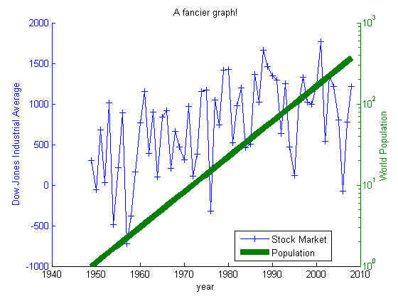
If handle graphics scare you, then you can still get nice plots. In the figure window, click the "View" menu and then "Property Editor". Now, click in various items in the figure to see menus relating to their properties. This is very powerful, but the disadvantage is that it is not automated, so if you close the plot, you must start over again.

There are many other graphic tools. For example, the linkdata button (also available on the command line as "linkdata on" and "linkdata off") will refresh the plot with new values whenever the variables that created it are updated (by default, this does not happen! plots are "frozen" with the current value of a variable).

FFT (Fast Fourier Transform)

You should refresh yourself on the FFT -- see a good textbook or the internet. It is often convenient to think of the FFT as a matrix; when the FFT operates on a vector of length N, we can instead think of a N x N matrix F that multiplies the vector. Of course, we don't usually do it this way because a matrix-vector multiplication takes O(N^2) operations, while the FFT exploits redundancies and takes O(N*logN) operations. Hence the name "Fast".

clear; clc;
N = 4;
F = fft( eye(N))
% Observations: F is a complex matrix.  And, a lot of the entries look
% similar.  Also, the matrix is (almost) unitary:
disp('F*F'' is:')
F*F'
disp('F''*F is:')
F'*F
disp('Is F symmetric? F - F.'' is:')
F - F.'
% It's not exactly unitary in this form because we don't get the identity,
% we get a constant (8) times the identity.  But this is of little
% importance, and in fact the IFFT (inverse FFT) will account for this
% constant.  Because F is complex, be very careful to distinguish adjoint
% (') from transpose(.')

F =
   1.0000             1.0000             1.0000             1.0000          
   1.0000                  0 - 1.0000i  -1.0000                  0 + 1.0000i
   1.0000            -1.0000             1.0000            -1.0000          
   1.0000                  0 + 1.0000i  -1.0000                  0 - 1.0000i
F*F' is:
ans =
     4     0     0     0
     0     4     0     0
     0     0     4     0
     0     0     0     4
F'*F is:
ans =
     4     0     0     0
     0     4     0     0
     0     0     4     0
     0     0     0     4
Is F symmetric? F - F.' is:
ans =
     0     0     0     0
     0     0     0     0
     0     0     0     0
     0     0     0     0

disp('F*I is:')
I = ifft(eye(N));
F*I

F*I is:
ans =
     1     0     0     0
     0     1     0     0
     0     0     1     0
     0     0     0     1

Now, let's take the FFT of something interesting.

N = 100;
t = linspace(0,2.7, N);
w = 3;              % linear frequency
y = sin(w*2*pi*t);
f = fft(y);

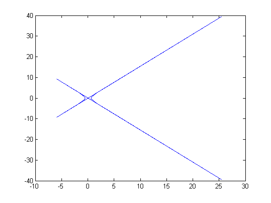
What if we plot f?

clf; plot(f)
% Huh?  Confusing.  This is because Matlab is plotting the Real part vs.
% the Imaginary part, which is not what we want.

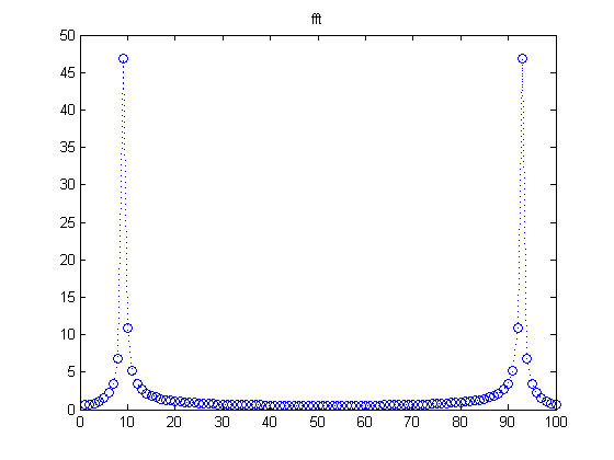
Instead, try this:

figure(1); plot( abs(f),'o:' ); title('fft')
% We're taking the FFT of a pure sinusoid.  Shouldn't we expect to have
% exactly one large component of the FFT, corresponding to the frequency of
% the sinusoid?  Yes and no.  First, notice the TWO peaks.  This is because
% our frequency w shows up, but so does -w.  For a real input signal, the
% FFT gives redundant information, and the first half of the signal is the
% complex conjugate of the second half, if we flip around the midpoint.

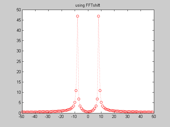
Matlab has a useful tool called "fftshift" that will do this flipping. To undo the effects of fftshift, use "ifftshift" (fftshift and ifftshift are either the same, or off by one, depending on if N is even or odd).

fftshift( 1:8 )         % to give an idea of what fftshift does
figure(2);
plot( [-N/2:0, 1:N/2-1], abs(fftshift(f)), 'ro:' )
title('using FFTshift')

ans =
     5     6     7     8     1     2     3     4

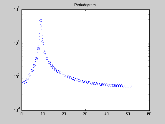
A useful way to plot:

semilogy( abs(f(1:N/2+1)), ':o' ); title('Periodogram')

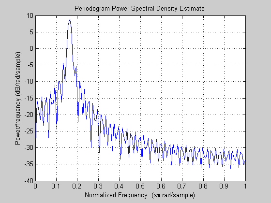
Or have Matlab do it for you:

periodogram(y)  % requires signal-processing toolbox
% If you tell it the sampling rate, it will use the correct units.

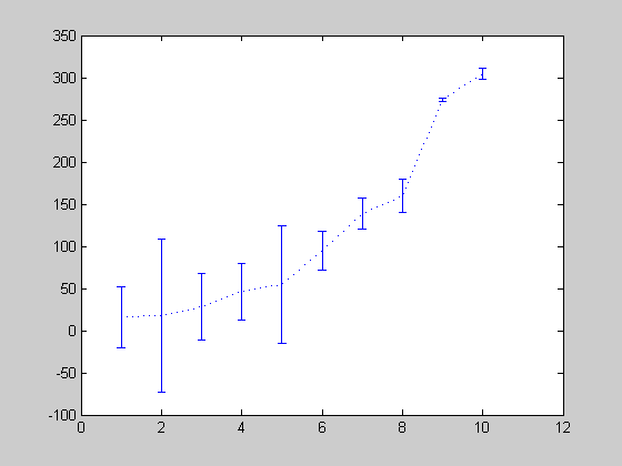
Making a plot with error bars

This is easy: use "errorbar" (see "help specgraph")

clear;clf;clc
x = 1:10;
y = 3*x.^2 + 20*randn(1,10);
err = 30*randn(1,10);
errorbar(x,y,err,':')