Lecture 5, ACM 11: advanced topics

Contents

Dealing with errors

There are two things we'd like to do with errors: (1) when we write our own code, we might want to "throw" an error, and (2) when Matlab generates an error, we might want to do something special. First, let's cover (1). When we throw an error, execution will stop. The simplest way to throw an error is just using "error('message')"

% error('This is an error message')

We can also give an ID to the message (this is useful if some program is going to do something about the error):

% error('lectureNotes:ErrMsg1','Another error message')

% The following is NOT valid:
% error('ErrMsg1','Another error message')  % need a ":" in the msgId

For objective (2), here's how to see some information about an error. We use the function "lasterror" as follows:

errInfo = lasterror
% The "stack" field is itself a structure,and contains information about
% where the error occurred (e.g. which file, which function, and which
% line).  This doesn't work when the code was executed in "cell mode"!

errInfo = 

       message: [1x102 char]
    identifier: 'MATLAB:lineBeyondFileEnd'
         stack: [6x1 struct]

Also as a part of objectve (2), we can handle Matlab's errors using "try" and "catch". Here's how:

try
    size( thisVariableDoesNotExist );   % because the variable doesn't exist,
                                        % Matlab will generate an error.
catch
    % If an error is thrown, then the code here will be executed:
    errInfo = lasterror;
    fprintf('Message identifier is: %s\n',errInfo.identifier);
    fprintf('Message string is: %s\n',errInfo.message);
    % and if we want to le the error continue, we can "rethrow" it:
%     rethrow( lasterror );
end

Message identifier is: MATLAB:UndefinedFunction
Message string is: Undefined function or variable 'thisVariableDoesNotExist'.

Warnings

If you put out a software package, then the "warning" command is very useful. You call it as "warning('message_id', 'message')". message_id should be in the form component:id (with the colon), otherwise it won't work properly:

warning('id','warning message')         % improper
warning('notes:id','warning message');  % proper

Warning: id

We can tell Matlab to ignore warnings. For example,

warning off all
warning on Simulink:actionNotTaken
% turns off all warnings except the Simulink:actionNotTaken warning
warning on all

or, turn off our own warning:

warning('off','notes:id')
warning('notes:id','warning message');  % no output now!

The "lastwarn" command works similarly to the "lasterror" command.

Parallel Computation and multithreading

Mathworks throws around several terms, so let's go over them first:

Release 2008 a and b:

 Parallel Computing Toolbox      -- useful for multicore machines

 Distributed Computing Server    -- useful for clusters

Releases 2006b to 2007b:

 Distributed Computing Toolbox   -- useful for multicore machines

 Distributed Computing Engine    -- useful for clusters

We won't cover the "Server/Engine" toolboxes, which are meant for clusters. Rather, we'll take a quick look at the PCT (or DCT, as it used to be called). The PCT is limited to a max of 4 processors, and they all have to be local (e.g. a quad-core machine, or two processors, both dual-core). This is an easy way to speed up your own code. The DCT, being simpler than the Server/Engine, is meant for what Matlab calls "distributed" computing, which is basically any kind of embarrasingly parallel computation (i.e. the nodes don't need to communicate). Mathworks refers to "parallel" computation as any more complicated parallel computing. In the "distributed" computing framework, there are two simple tasks: (1) each computer independently computes, or (2) each computer independently holds some portion of a variable in memory. The new PCT is more powerful than the old DCT, but still not meant for clusters.

The simplest method for distributed computing is the "parfor" command, which is like a "for" loop, except it distributes different iterations to different processors. You first ask for a pool of processors using "matlabpool" (this make take 10 or more seconds). Even if you are on a single-core processor, if it has hyperthreading, it can emulate multiple processors, and perhaps even have a speed benefit, although this is unlikely. At the end, call "matlabpool close". Other useful commands: pmode.

Example of explicit distributed computation:

tic; matlabpool open 2
t = toc; fprintf('Took %.2f seconds to open the "pool"\n',t);

A = randn(300);N=200;         % this is faster with the "parfor"
% A = randn(1000); N = 2;       % this is barely faster with "parfor"
                                % because there is a lot of memory copying
tic;
for i = 1:N
    svd(A);
end
t = toc;
fprintf('Operation took %.2f seconds with normal "for" loop\n',t);
tic
parfor i = 1:N
    svd(A);
end
t = toc;
fprintf('Operation took %.2f seconds with "parfor" loop\n',t);
matlabpool close

Starting matlabpool using the parallel configuration 'local'.
Waiting for parallel job to start...
Connected to a matlabpool session with 2 labs.
Took 16.80 seconds to open the "pool"
Operation took 21.46 seconds with normal "for" loop
Operation took 12.05 seconds with "parfor" loop
Sending a stop signal to all the labs...
Waiting for parallel job to finish...
Performing parallel job cleanup...
Done.

If we made a simple matrix multiplication call, then the parfor has no advantage, because matrix multiplication is a BLAS operation, and Matlab already multithreads this (usually).

Implicit vs Explicit multithreading

The above is an example of explicit multithreading -- it affects user-written code. Since release 2007a, Matlab has had an implicit multithreading option, and since 2008a, it has been turned on by default. To turn it on/off, go to "File>> Preferences>> General:Multithreading". You can also vary the number of processors from the command line with "maxNumCompThreads".

With multithreading turned on, Matlab will run multithreaded versions of LAPACK and BLAS -- the subroutines that do matrix operations. If you have installed another version of BLAS, and told Matlab to use that, then it may or may not be multithreaded (it probably can be, but with a bit of extra work).

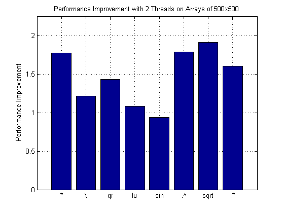
To see if this can speed up computations on your computer, run the demo "multithreadedcomputations". See also "bench".

multithreadedcomputations

Time for 1 thread  = 0.061 sec
Time for 2 threads = 0.031 sec
Speed-up is 1.954

function [meanTime names] = runAndTimeOps
% Time a number of operations and return the times plus their names.
% Other functions can be inserted here by replicating the code sections.

% Set parameters
numRuns = 10;               % Number of runs to average over
dataSize = 500;             % Data size to test
x=rand(dataSize,dataSize);  % Random square matrix

% Matrix multiplication (*)
func=1; % Initialize function counter
tic;
for i = 1:numRuns
    y=x*x;                  % Call function
end
meanTime(func)=toc/numRuns; % Divide time by number of runs
names{func}='*';            % Store string describing function
func=func+1;                % Increment function counter

% (snipped output for brevity) 

% Element-wise multiplication (.*)
tic;
for i = 1:numRuns
    y=x.*x;                 % Call function
end
meanTime(func)=toc/numRuns; % Divide time by number of runs
names{func}='.*';           % Store string describing function
func=func+1;                % Increment function counter

An example of implicit multithreading (this is just a BLAS call):

clc; A = randn(1200);
for n = 1:2
    maxNumCompThreads( n );
    tic; A^2; t = toc;
    fprintf('On a Centrino Duo processor, using %d threads, time is %.2f\n',n,t);
end
% I get about 1.50 seconds vs 0.83 seconds, so it is an improvement
maxNumCompThreads('automatic');

On a Centrino Duo processor, using 1 threads, time is 1.49
On a Centrino Duo processor, using 2 threads, time is 0.82

LAPACK and BLAS

Matlab has its own version of LAPACK and BLAS. These are called libmwlapack and libmwblas. If you have a version of BLAS that you prefer, you can tell Matlab to use it. See the documentation.

LAPACK is a set of routines for linear algebra. BLAS is a set of routines for vector-vector ("level 1"), matrix-vector ("level 2") and matrix-matrix ("level 3") operations. There are many versions of BLAS, often released by Intel and AMD, that are optimized for particular CPUs. LAPACK calls BLAS, so LAPACK is machine-independent. Intel's BLAS is part of their Math Kernel Library (MKL). Other forms of BLAS: the reference (un-optimized) BLAS at netlib.org; ATLAS, an auto-tuning form of BLAS; GOTO BLAS, a version devloped by Kazushige Goto.

LAPACK was first used in Matlab in 2000 (release 6), replacing LINPACK and EISPACK. LINPACK only used level-1 BLAS, and EISPACK didn't use BLAS at all, while LAPACK uses full level-3 BLAS.

FFT

Starting in 2000 (release 6), Matlab calls a special version of fftw for FFT calculations. It deals with the fftw "wisdom" automaically, although you can control these settings a bit (in particular, you can have it do an exhaustive search for the best method). You should note that, for a particular size vector, the first call to fft is always slower than subsequent calls, due to calculation of the wisdom (although, probably not for powers-of-two, where the "wisdom" is obvious).

N = 100000 + round( 100 * rand );
tic; fft(ones(N,1)); t = toc;
tic; fft(ones(N,1)); t2 = toc;
fprintf('On first call, for size %d,\n\t the FFT took %.2e sec, and %.2e on 2nd call\n',...
    N,t,t2);

On first call, for size 100059,
	 the FFT took 8.88e-001 sec, and 3.12e-002 on 2nd call

Memory limits

Type "memory" to see how much memory is available to Matlab. On 32-bit windows, there is a 2 GB process limit, independent of the physical memory (this can be raised to 3 GB by changing boot.ini). You can reduce Matlab's memory footprint by 150 to 400 MB by starting it without the java virtual machine (use the command "matlab -nojvm"), although you can't use the editor. Starting with the desktop ("matlab -nodesktop") doesn't help much. BTW, note that on linux, to make a shortcut to Matlab work on the desktop, you must use the command "matlab -desktop".

clc; memory

Maximum possible array:            1005 MB (1.054e+009 bytes) *
Memory available for all arrays:   1336 MB (1.401e+009 bytes) **
Memory used by MATLAB:              476 MB (4.995e+008 bytes)
Physical Memory (RAM):             2046 MB (2.145e+009 bytes)

*  Limited by contiguous virtual address space available.
** Limited by virtual address space available.

Functions within functions

Subfunctions can come in two flavors:

======= Flavor 1: ============

% function mainFunction
% [body of mainFunction]
%
% function subFunction
% [body of subFunction]

======= Flavor 1, variation (same effect, different syntax) =====

% function mainFunction
% [body of mainFunction]
% end
%
% function subFunction
% [body of subFunction]
% end

In flavor 1, the subFunction is only visible to the mainFunction. In all other respects, it acts like a normal function. In particular, subFunction can't see any of the local variables in mainFunction.

======= Flavor 2: ============

% function mainFunction
% [body of mainFunction]
%
% function subFunction
% [body of subFunction]
% end
%
% end   % this refers to mainFunction, not subFunction

Now, subFunction is not only local to mainFunction, but it can "see" all the local variables of mainFunction. This can be very useful sometimes!

Persistent variables in functions

Similar to "static" variables in C/C++. These variables are not destroyed after the function is called!

example:

dct();      % reset the counter
for i = 1:5, dct( ones(10,1) ); end
fprintf('DCT has been called %d times since it was last reset\n',dct() );

% is "isempty" to check if the variable hasn't yet been created.
% Everytime you edit the file, or open/close matlab, the persistent
% variable is cleared.

DCT has been called 5 times since it was last reset

Here is code for dct.m

Private subdirectories

Any files located in a subdirectory called "private" are only visible to the files located in the immediate parent directory. This is useful for software releases with subfunctions that shouldn't be visible to the user. Also, subdirectories in the form "@className" are treated specially: they instruct Matlab to use the subfunctions in that directory if the input is of the type className. For example, to multiply arrays using "times", there are different routines depending on the type of data. Matlab automatically uses the correct one. You can see the routines by using "which -all":

clc;
which -all times

built-in (C:\Program Files\MATLAB\R2008a\toolbox\matlab\ops\@single\times)         % single method
built-in (C:\Program Files\MATLAB\R2008a\toolbox\matlab\ops\@double\times)         % Shadowed double method
built-in (C:\Program Files\MATLAB\R2008a\toolbox\matlab\ops\@char\times)           % Shadowed char method
built-in (C:\Program Files\MATLAB\R2008a\toolbox\matlab\ops\@logical\times)        % Shadowed logical method
built-in (C:\Program Files\MATLAB\R2008a\toolbox\matlab\ops\@int32\times)          % Shadowed int32 method
built-in (C:\Program Files\MATLAB\R2008a\toolbox\matlab\ops\@int16\times)          % Shadowed int16 method
built-in (C:\Program Files\MATLAB\R2008a\toolbox\matlab\ops\@int8\times)           % Shadowed int8 method
built-in (C:\Program Files\MATLAB\R2008a\toolbox\matlab\ops\@uint32\times)         % Shadowed uint32 method
built-in (C:\Program Files\MATLAB\R2008a\toolbox\matlab\ops\@uint16\times)         % Shadowed uint16 method
built-in (C:\Program Files\MATLAB\R2008a\toolbox\matlab\ops\@uint8\times)          % Shadowed uint8 method
C:\Program Files\MATLAB\R2008a\cvx\builtins\@cvx\times.m                           % Shadowed cvx method
C:\Program Files\MATLAB\R2008a\toolbox\matlab\timeseries\@timeseries\times.m       % Shadowed timeseries method
C:\Program Files\MATLAB\R2008a\toolbox\distcomp\parallel\ops\@distributed\times.m  % Shadowed distributed method
C:\Program Files\MATLAB\R2008a\toolbox\shared\statslib\@categorical\times.m        % Shadowed categorical method
C:\Program Files\MATLAB\R2008a\toolbox\symbolic\@sym\times.m                       % Shadowed sym method

Startup file

If a file called "startup.m" exists in a directory in your path, it will be run everytime matlab loads. This is a nice way to load any software packages you want, or define variables, or change the path. Remember, the "path" is order-sensitive, so use "addpath ... -end" or "addpath ... -begin" (default) to add a path to the appropriate place in the list.

Handy utilities

Matlab has builtin functions like "zip", "tar", "ftp", "sendmail", "urlread", ... See "help iofun".

Handle graphics

See the example file markerColor.m. This shows how to use "set", "get", "gca" etc. If you have a handle h, then "set(h)" shows the default values for that type of handle, and "get(h)" shows the current state of all the values.

close;clear;clc
x = 1:20;
h = plot( x, x.^3, 'ro' );

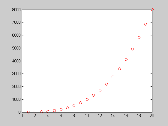
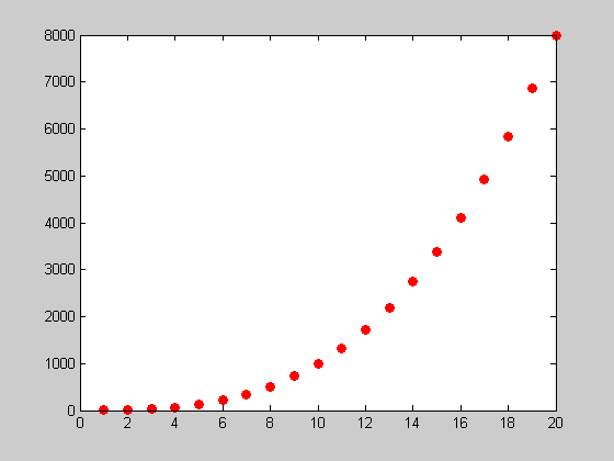
This function will get the handles to the current axis (with "gca"), look for all "children" objects that have the property "markerFaceColor", and set this property to the color of the marker (since, by default, the edge of the marker and the interior/face of a marker are different colors -- the interior/face is always white, by default).

markerColor

edit markerColor

Dealing with different workspaces

The command "who" will tell me what variables are in the current workspace. But in a function (as opposed to a script), I don't have access to this workspace. If I still need access, I can use the "callin" (and "evalin") functions. For example, if I want a modified version of "whos" (call it "whoss") that lists information in a nicer format, then I use the "callin" format.

A = randn(300);
B = randn(600);
clc;
whoss

	A                   	703.1 Kb
	B                   	2.7 Mb
	h                   	8
	x                   	160

edit whoss

Here is code for whoss.m

A similar useful tool is the "builtin" command. If you have a function with the same name as a Matlab function, and shadows the Matlab function (type "which -all NAME" to see all functions with the name "NAME"), then the "builtin" command will call the original Matlab function.

Just-In-Time accelerator

This makes up a little bit for the problems with an interpreted language (basically, it compiles bits of code just before they are run). It is undocumented, and changes with every release; you are not supposed to build your code assuming that it will be accelerated! Because Matlab is not strongly-typed, and for other reasons, it is not easy to have a JIT, so it only accelerates in some cases. See the example file. It only works in m-files, not from the command line, and it doesn't always work in cell mode. Rather tricky! But, moral of the story, for "for" loops, make your iterated variables simple! It used to be, prior to 2006, that the "profiler" feature would give recommendations on how to change your code so that it can be accelerated. Sadly, they removed this feature.

edit test_JIT.m

Here is code for test_JIT.m

Graphical user interface

Use the GUIDE design tool. It's pretty easy, but you have to use handle graphics. For example,

working_memory

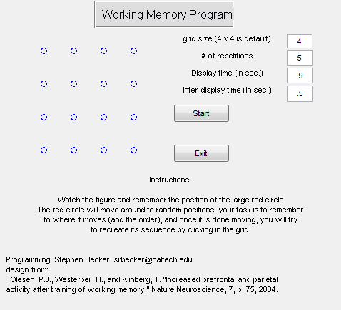
The code for the above GUI is working_memory.m and working_memory.fig

Matlab from the command line

There are several ways, e.g.

% matlab -nodisplay >& outputFIle << EOF
% [commands in matlab]
% EOF       (cntrl-d)

% or
% matlab -nodisplay < inputFile &

% or
% matlab -nodisplay -r "disp('a Matlab command'); exit"

% the above requires the "exit", and you can't put it in the background or
% else it stops and won't restart in the background.

% for help, type "matlab -help"

Debugging

Debugging in Matlab is most useful in conjunction with "breakpoints." To add a breakpoint into a line of code, just click the horizontal line to the left of the line of code. It should turn into a red dot. The dot turns gray if the code has been changed and not saved. When you run the code, the execution pauses at the breakpoint everytime it reaches the line. The Matlab command menu now has a different look to it: "K>>". You can see the local variables to the function, and hopefully piece-together what went wrong! To step through the code, or let it run, see the various options (and the shortcuts) in the "Debug" menu of the editor. You can also control these with commands, e.g. to quit the debugger, use "dbquit".

In particular, in the Debug menu, the "Stop if Errors/Warnings" will let you tell the debugger to go into debug mode at the occurence of any error. This is extremely useful. You can also enable this as a command via "dbstop if error" (but accessing it via the menu gives you a fuller view of all the options available).

It is also possible to do "breakpoints" as lines of code. For example, insert the command "keyboard" and Matlab will effectively enter debug mode whenever this code is run. For example, you may have a statement like:

myVariable = 10000;

if myVariable < 20
    % everything is good
else
    % something went wrong.  Enter debug mode to examine the states of the
    % variables:

%     keyboard;
end
% to get out of keyboard mode, type "return" or "dbquit".

Profiling -- finding the bottlenecks in your code

Matlab has the simplest performance analyzing tool ever! Open up a m-file, then select "Open Profiler" from the "Tools" menu (you can also call it from the command line). In the top, it says "run this code", and either use the suggestion or give it your own command (note: you cannot profile a single cell; it must be a full m-file script, or a function). Then wait, and look at the results. It gives a breakdown in terms of functions and lines of code, and by how often the code was called and how long was spent in the computation. Nice!

profile on
dct( ones(10000,1) );
profile off
profile viewer

mlint -- letting the computer tell you what you can improve

"mlint", named after the original "lint" program, is designed to find weaknesess in the code (but not errors -- those are easily found). You can run the command "mlint" to get a list of suggestions. Or, look at the mlint section from the profiler results. Or, in the editor, the little colored items on the right, near the scroll-bar, represent mlint suggestions. In the latest releases, mlint gives you suggestions even as you type! Many of these suggestions are very useful, while others are not.

Matlab report-generator

This is how all the notes and homework solutions for the class were generated. You write an m-file, and then call the report-generator which will run the commands in the m-file and insert the comments and results into a document (e.g. html, xml, pdf via latex, ...). You can insert latex commands into comments like:

It's a bit picky, and takes getting used to. There are many advanced options (e.g. only re-running part of the code, using your own style-sheets) that I won't cover.

For printing out homeworks, the most useful way to stylize your code is to select "Styled text" (or "color") under "Page Setup" from the editor's "File" menu. This puts comments in italics, and is much nicer to read.

web file:///C:/Users/Stephen/Documents/MATLAB/html/lecture5.html#41

Matlab mex files

"mex" can refer to several things in Matlab. The simplest case: you use mex files to compile a C/C++/fortran code into a "mex" file that can be called from Matlab. There are many Matlab functions you can use (include "mex.h" in the file), and the help menu documents them. Basically, any function called "mx..." (e.g. "mxCreateDoubleMatrix") will do something in C/C++/fortran, while any function called "mex..." will do something back in the Matlab environment.

There are also MAT files, which are functions provided to insert into non-Matlab code that will read and write from .mat files.

It is also possible to use the Matlab Engine from another programming language. You must have Matlab installed (it need not be on the local computer, but it must be on a networked computer) to use this.

For compiling, Matlab has its own compiler, "lcc", but you can use others as well. Run "mex -setup" to select which one you like. To compile a mex file, use the "mex" command. It takes many options similar to a standard compiler, but it also does some things automatically (determined by the script setup by running "mex -setup"), such as include the directory where "mex.h" is located, link to the mathworks LAPACK libraries, etc. For installing 3rd party programs, if they were not designed robustly or you have a weird computer setup, it may be necessary to adjust system environment variables. On linux, for example, you may need to change "LD_LIBRARY_PATH" to point to where your shared libraries are. Matlab can set the current envirnoment variables using the "setenv" command.

"mex -setup" will put the configuration file in the user's "prefdir" (type "prefdir" to see where this is on your computer).

Most Windows systems don't have a default C compiler installed; however, Microsoft's Visual Studio is free for students (via the DreamSpark program: see https://downloads.channel8.msdn.com). For Linux and Mac, the gcc suite of compilers is free.

% This example is located here:
p = fullfile(matlabroot,'extern','examples','mex');
% On Windows Vista, I need to copy these files to a place on the filesystem
% where I have permission to write!

% mex -setup        % you only need to do this once ever!
edit yprime.c
mex yprime.c
which yprime    % the mex file (.mexw32) overshadows the .m file
yprime(1,1:4)
% the Help documentation is still in yprime.m
% On different OS, the mex file will have different endings (e.g. .macosi
% for Intel Mac, or .mexglx for 32-bit Linux).

C:\Users\Stephen\Documents\MATLAB\yprime.mexw32

ans =

    2.0000    8.9685    4.0000   -1.0947

Matlab Compiler (MCR)

This is a toolbox that allows one to write code that uses Matlab, but can be compiled to include the Matlab features and be independent of Matlab in the future (i.e. for commercial release, or for an embedded device). We won't cover this.

why?

Matlab always has the answer:

clc
for i=1:5
    why
end

To fool some tall and young and not very bald kid.
The smart and terrified mathematician told me to.
Some smart hamster insisted on it.
Barney told me to.
Some terrified good hamster wanted it that way.

Published with MATLAB® 7.6