ACM11: supplemental ODE notes

Contents

A predator-prey example

The class predator-prey model is the Lotka-Volterra Equation. For background, please see http://en.wikipedia.org/wiki/Lotka–Volterra_equation This models the populations of two species, say, humans and raptors. The population sizes change based on different factors. For humans, the human population increases faster if there is a bigger population (hence we have exponential growth), but the population is decreased if the raptor population is large, due to raptor-attacks. For raptors, a large population is bad, because it means more competition for food. But a large human population is good for raptors. Hence, we propose the following simple model for the human (h) and raptor (r) populations:

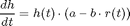
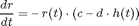
where a, b, c and d are parameters of the model.

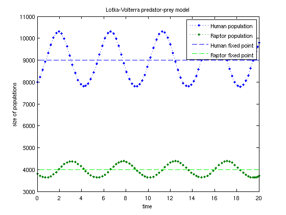
Furthermore, the system has two fixed points: a stable one at h(t) = r(t) = 0, and an unstable one at h(t) = c/d and r(t) = a/b. These fixed points are not important to our problem. First, we'll solve this ODE for a fixed amount of time.

% Pick some parameters
a = 2; b= .0005;
c = .9; d = .0001;
t_initial = 0;
t_final = 20;
t_interval = [t_initial, t_final];
human_initial = 8000;
raptor_initial = 3800;
initialConditions = [human_initial; raptor_initial]; % a column-vector

% Here is the code for predPrey.  This is in a file called "predPrey.m":

% function dy = predPrey(t,y, a, b, c, d)
% dy = zeros(2,1);    % a column vector
% human = y(1);
% raptor = y(2);
% dy(1) = human * ( a - b*raptor );
% dy(2) = -raptor * ( c - d*human );

% Setup the right-hand-side of the ODE.  This solves for raptors and humans
% at the same time, since the variables are coupled.  I want to use the a,
% b, c and d parameters defined above, so I can "freeze" those in like
% this:
myOdeFun = @(t,y) predPrey(t,y, a,b,c,d);
% Now t and y are variables, and a, b, c and d are fixed parameters.

% If the above lines are confusing, then there's a workaround.  We could
% set the values of a, b, c and d inside the predPrey.m function.  In that
% case, then we would define myOdeFun as:

% myOdeFun = @predPrey;


% Now, call Matlab's solver:
[T,Y] = ode45( myOdeFun, t_interval, initialConditions );

% And plot the results
plot(T,Y,'.:')
line( t_interval, c/d*[1,1], 'color','blue','linestyle','--')
line( t_interval, a/b*[1,1], 'color','green','linestyle','--')
legend('Human population','Raptor population','Human fixed point',...
    'Raptor fixed point');
xlabel('time'); ylabel('size of populations');
title('Lotka-Volterra predator-prey model');

Putting in cutoffs

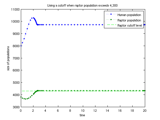
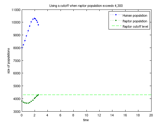
Suppose the US Dept. of Fish and Wildlife Management is concerned about the raptor population. Specifically, raptors will be considered an "endangered species" unless their population rises above 4,300. For our modelling, we only care about raptors when they are "endangered", and we might wish to stop our model once the population rises over 4,300. There are two things we can do. First, we can change the ODE to make it become very simple once we reach 4,300. The benefit of this is that the ODE solver will realize the ODE is very simple and will take very large time-steps. The second method is to explicitly tell Matlab to stop computation once the threshold has been reached. First, we'll go over method one:

% Method one, with the same setup as before.  We modify myOdeFun a bit:
myOdeFun = @(t,y) ( y(2)<4300 ) .* predPrey( t, y, a, b, c, d);

% Now, call Matlab's solver exactly as before:
[T,Y] = ode45( myOdeFun, t_interval, initialConditions );
% And plot the results
plot(T,Y,'.:')
line( t_interval, 4300*[1,1], 'color','green','linestyle','--')
legend('Human population','Raptor population','Raptor cutoff level');
xlabel('time'); ylabel('size of populations');
title('Using a cutoff when raptor population exceeds 4,300');

% We can see that the spacing of the time-grid changes after the cutoff.
% The data after the cutoff is incorrect, but we don't care about that
% data.

Putting in cutoffs (method 2)

For this, we use the "Events" property; type "doc odeset" for details. The idea is that, upon some user-defined event, the ODE solver will change behavior. For example, suppose we model a bouncing ball. In the air, the behavior is determined by gravity, but the direction of motion switches everytime it hits the ground. To do this, we pass the ODE solver a function (say, "events"), with the form [value,isterminal,direction] = events(t,y). In the case of a ball dropping, the "value" of the event would be the position of the ball; when value = 0, the "event" has occured. If "isterminal" is true, then the ODE will stop when the event occurs, otherwise it will simply record the fact and keep solving. The "direction" parameter is not important to us, and we can ignore it.

% the events function is in the file "events.m":
% function [value, isterminal,direction] = events(t,y)
% isterminal = double(true);
% direction = 0;
% value = double(y(2) < 4300);

% now, use the original "myOdeFun":
myOdeFun = @(t,y) predPrey( t, y, a, b, c, d);

% This is where the magic occurs:
opts = odeset('Events', @events );

% Now, call Matlab's solver, AND give it "opts":
[T,Y] = ode45( myOdeFun, t_interval, initialConditions, opts );
% And plot the results
plot(T,Y,'.:')
line( t_interval, 4300*[1,1], 'color','green','linestyle','--')
legend('Human population','Raptor population','Raptor cutoff level');
xlabel('time'); ylabel('size of populations');
title('Using a cutoff when raptor population exceeds 4,300');

Further MATLAB references

In the Matlab help menu under the "Contents" tab, select MATLAB >> Mathematics >> Differential Equations >> Initial Value Problems... >> Examples: Applying the ODE...

This Matlab help topic is also online at various sites on the web.

Published with MATLAB® 7.2