Iterated Function Systems

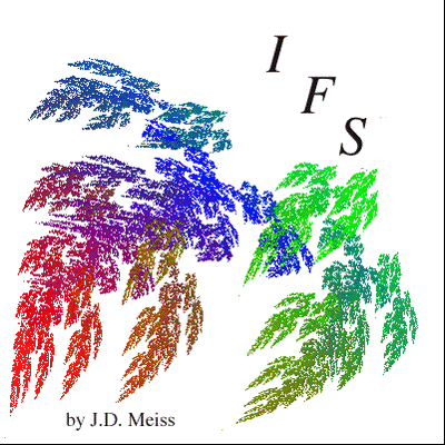
IFS is a Macintosh application for drawing the fractals created by iterated function systems. A standard example is the "Sierpinski gasket" which is the icon for the application. IFS requires MacOS 10.6 or later.

IFS version 2.2.1 Mac OS X 10.6-10.14 (Intel processor)

Download

What it does

Iterated function systems are dynamical systems defined by a set of n mappings f_i. In the case of IFS, we allow the f_i to be affine maps of the plane:

f(x) = A x + b

where A =[[a,b],[c,d]] is a 2x2 matrix and b is a two dimensional vector. If 0 <|det(A)| < 1, then f is a contraction, and any point under iteration

x´= f(x)

approaches the unique fixed point x = - A^-1 b.

An iterated function system allows the choice of any of the n affine maps with probabilities p_i for the iteration, thus

x´ = f_i(x) with probability p_i

In the program, n is initially 3, and the p_i = 1/3, so that it is equally likely to have any one of the f_i. An iterated function system with contractions f_i has a unique attractor S that satisfies the equation

S = f₁(S) U f₂(S) U … f_n(S)

Often this attractor is fractal in structure. Making pictures of these attractors is the job for IFS.

Using IFS

Choosing a transformation The Sierpinski triangle is defined by the affine transformations f_i with A = [[0.5,0,],[0,0.5]], and b₁ = (0,0), b₂= (0,0.5) and b₃ =(0.5,0). To obtain this with the program choose "Sierpinski Relative" from the "Show" menu, and type in "0" for each of the symmetry elements.

The Sierpinski relatives have f_i given by the same matrices as before, but composed with one of the 8 symmetry transformations of the square. We let D₀ be the identity, D₁ be the rotation by 90 degrees, and D₄ be the reflection about the x-axis. The group elements are defined as

D₀ = I
D₁ = [[0,1,],[-1,0]]
D₂ = D₁²,
D₃ = D₁³,
D₄ = [[1,0],[0,-1]],
D₅ = D₄D₁,
D₆ = D₄D₂,
D₇ = D₄D₃

With the "Sierpinski relatives" menu, you can choose a symmetry element for each of the f_i. This gives 2⁸ possible attractors, of which 232 are distinct structures. There are four distinct topological types among these structures—to learn more about this see [Robins, 1997].

The second way to choose the transformations f_i, is to use the "Similarity transformations" menu item. A similarity transformation is a rotation composed with a scaling. To choose each transformation you click twice in the plot window. The first click sets the vector b, which is the iterate of the origin. The second click chooses the position which the point (1,0) iterates to. So your second click chooses the angle through which the x-axis is rotated, as well as the length to which it is scaled. Hold down the option key to reflect the similarity (det(A) < 0). To choose all n-transformations, you must choose two points in the plot window for each.

Finally, you can choose a general affine transformation with the "Affine Transformation" menu item. The affine transformation is fixed by 3 vectors, the two columns of A and the vector b. A first click in the plot window fixes b, the second fixes the first column of A (setting the image of the point (1,0)), and the third click fixes the second column of A (setting the image of the point (0,1)).

The Menus

• The Show Menu

  The program starts up by displaying the orbit of the origin under 50,000 iterations with randomly chosen f_i. We use the basic "srand" function built into C for the pseudo-random number generator, so don’t expect sophisticated statistical properties.

  You may also show "recursive" iteration. This means to show the image of the unit square (0,0) x (1,1) under all possible sequences of iterations f_i f_j f_k…, out to some level l. Initially l = 3.

  You may also view just the first iterate of the unit square under each of the transformations by selecting the "Show: Affine Transformations" menu item.

  Finally, if there is a picture in the clipboard, you may paste it into the plot window, and show this. However, this is not working to well with the other parts of the program yet.

• The Set Parameters Menu

  You may set the number of random iterations (N = 50,000 initially), the number of levels of the recursive iteration (L=3 initially), choose the number of transformations, (n=3 initially) and the probabilities p_i (p_i = 1/n initially) with the "Set Parameters" menu.

• The Windows Menu

  Apart from the usual commands,you may zoom in or zoom out of the plot by selecting the appropriate menu items. To zoom, drag a rectangle in the plot window.

  You may also choose the colors for each transformation f_i in this menu. The colors are used to display the color of each point x_t after t iterations according to the simple IFS for colors: color´ = 0.5 (color + color(f_i)). Thus if we iterate for a long time with f₁, then the color of the point approaches the color of f₁.

Suggestions and comments welcome

This is a rudamentary version a MacOS Application, and as such is to be thought of as a rough outline of a complete program. Let me know your thoughts about how the program should improve!

This program is free for noncommercial use, but the copyright remains with the author. It may not be sold or included in any commercial collection without the express written approval of the author.

Known Problems (might be called bugs)

• On some computers, when you drag the resize box, or drag to graphically create an affine transformation, the old rectangles are not completely erased. In some cases the window background goes black. I believe this has something to do with my mixing of OpenGL and Quickdraw graphics calls. But I haven't isolated it yet.

References

Barnsley, M. (1988). Fractals everywhere. Boston, Academic Press.
Peitgen, H. O., H. Jürgens, et al. (1992). Chaos and Fractals. New York, Spinger-Verlag.
Robins, V., J. D. Meiss, et al. (1997). "Computing Connectedness: an exercise in computational topology." Nonlinearity 11: 913-922.
Robins, V., J. D. Meiss, et al. (1999). "Computing Connectedness: Disconnectedness and Discreteness." Physica D 139 276-300.