About StdMap |
|
|
The piecewise linear map is just one of 13 maps that you can iterate with StdMap. |
For a tutorial on StdMap see my article Visual Explorations of Dynamics. There are three “help” facilities in the program. If you turn on “Give Helpful Tips” by checking the menu item (it is on by default at launch), I attempt to give you more information about what is happening. For example when you choose a new map its formula is written to the text window. Secondly, if you let your mouse hover over a menu item or control in a window or dialog then “help tags” will pop up to give you a bit of help. Finally, these help files are availiable from the Help Menu. However, they are not very extensive as of yet.
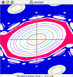
Standard Maps displays the dynamics of several “area preserving” mappings. It will also find periodic orbits, cantori, and stable and unstable manifolds of any (symmetric) periodic orbit, and allow you to iterate arbitrary curves.
By default the program starts up in random iteration mode (you can turn this off by unchecking "Give Helpful tips" in the Change menu. Then the default startup mode is to not iterate). In random mode, a new initial condition will be chosen--yes--at random ever second or so (the number of iterates can be changed if you select Find-›Random Initial Condition).
If you would like to choose your own initial condition, simply click in the plot window (is is called "untitled" unless you save the file). The iteration begins from the point you click and continues ad infinitum. Iteration can be stopped by selecting Find-›Iterate and re-started by selecting it again. Click at a new location to launch a new initial condition.
There are several iteration modes. For example, if you use the Find -›SingleStep menu, then the map is iterated once each time you hit the spacebar, and the orbit is plotted wiht a small box instead of a single pixel. This is a good way of showing the iterations step by step.
One fun thing to do is to iterate the stable an ustable manifolds for a periodic orbit. To do this select Find -›Stable Manfold. Choose the periodic orbit (p=0, q=1 is the fixed point), and a sign 1 or -1 to decide which direction you would like the manifold to go (up in y or down in y). The program will allocate a large pointer to save the points on the curve, so wait a few seconds while it does this. Then hit the space bar (or click on the Iterate button) to iterate the manifolds one step.
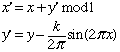
Since the map is periodic in x with period one, we take x mod 1 to wrap it into the interval [-0.5, 0.5). Thus the standard map is really a map on the cylinder. There are two topological types of maps in the program. The second is exemplified by the Hénon map
New maps are selected in the Maps menu. Each of them is technically a "reversible, area-preserving map." The last two maps--the "Two Wave Flow" and "Force Duffing" are actually "time-one" maps of non-autonomous differential equations.
An orbit is periodic if it returns to itself after q steps. You can find peridic orbits using the Find menu. There are also more exotic orbits that can be found: homoclinic and quasiperiodic (using the Farey Path) ones.
Each orbit also has a color associated with it. You can change the color for the next orbit on the Window menu. You can also change the color of existing orbits in the Edit Orbit List dialog.
There are many options in the Change menu. Many of them (showing or not showing the axes, showing or not showing the number of iterates, etc.) are saved in the applications preference file (in your Library/Preferences folder), so that when you start-up the program again you don't have to readjust things. I also save the window sizes and positions, so set those up as you like.
If you save a map to a file, the program will save the map parameters and the current picture to the file. You can also--by checking the box "Save complete list of iterations"--save the list of points that make up each orbit. Take care here as this can result in very large files. The resulting files are text files, and can be opened with any text editor, though the picture (saved as a PICT resource) will usually be ignored. You can also copy the current plot to the clipboard using Edit-›Copy. The resulting picture can be pasted most anywhere. Text in the text window is also freely editable.